To demonstrate curve fitting using MATLAB.

Aim: To write a code in MATLAB to demonstrate curve fitting.

Objectives of the project:

• To write code to fit a linear and cubic polynomial for the given temperature vs specific heat data.
• To plot the linear and cubic fit curves along with the raw data points.
• To write a code to demonstrate splitwise curve fitting method.

Curve fitting: Curve fitting is a process of obtaining a mathematical function that best describes the given series of data points. When this obtained mathematical function is plotted, we expect it to closely match or fit with the curve that represents the original data points. Hence, the fitted curve or the mathematical function can be used to aid better data visualization, then the function can further be extrapolated to obtain a fair prediction of the future trend based on the past data, or it can also be used to interpolate to find values within the curve where no data is available.

The most common form used to fit a series of data points is by fitting a function in the form y=f(x). Where f(x) is a polynomial function. The polynomial function can be of the order ‘n’. When n = 1, the first-degree polynomial equation is that of a straight-line equation.

y = ax + b

This straight line would connect any two points, hence a first-degree polynomial equation is an exact fit through any two points with distinct x coordinates.

When n = 2, the second-degree polynomial equation would fit a simple curve of three points.

y = ax² + bx + c

When n = 3, the third-degree polynomial equation would fit a curve with four points, and the equation would be as follows,

y = ax³ + bx² + cx + d

Therefore, if ‘n’ is the degree of the polynomial equation, then it would fit a curve with ‘n+1’ points.

Limitations of using a polynomial function: Some of the limitations of using a polynomial function to fit a curve is increasing the degree of a polynomial function does not always result in a better fit. Higher-order polynomials tend to be oscillatory between the data points, which is explained as Runge’s Phenomenon. This leads to a poorer fit to the data. Hence, we might have to use different techniques to fit the data depending on the problem.

We should also acknowledge the fact that the polynomials are unbounded and oscillatory in nature. Hence they are not suited for extrapolating data based on past data. However, we can use the function to interpolate data at undefined data points.

Errors associated with curve fitting: When we attempt to fit a curve with a polynomial function, we may encounter errors or deviations of the points in a fitted curve from the original curve. Hence there are four quantities that help us measure these deviations and help us determine the goodness of a fit. They are:

1. The sum of squares due to error (SSE)
2. R-Square
3. Adjusted R-Square
4. Root mean squared error (RMSE)

Each of them is discussed as follows:

The sum of squares due to errors (SSE): The sum of squared errors is basically the summation of squared values of the deviations/errors of the predicted values from the original values. It is a measure of how well the independent values fit the data.

SSE is given by:

`SSE = ∑_(i=1)^n Err(i)^2`

We assume the proposed equation is n^th degree polynomial of the form,

f(x) = a1 + a2•x + a3•x² + … + an•x^n-1

When we differentiate the SSE with all the coefficients of the polynomial function f(x) and equate it to zero, we can find the minima and the value of that coefficient.

`[∂SSE/∂a1=0,∂SSE/∂a2=0, ... ,∂SSE/∂an=0]`

Upon solving the multiple systems of equations, we can find the values of all the coefficients. Thus, the obtained polynomial equation can be used to fit the curve.

R-Square: R-square is the square of the correlation of between the original response values and the predicted response values. It basically means that if the value of R-Square is higher, it gives a better fit. Similarly, a lower value of R-Square gives a lousier fit. R-Square values range from 0 to 1. Hence,

The value of 0 would correspond to the worst possible fit for the given data set and

The value of 1 would correspond to the best possible fit for the given data set.

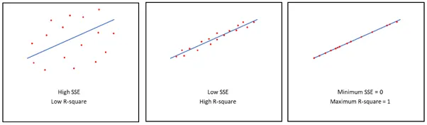
The R-Square is calculated as follows:

If y = f(x) is the fit curve, then the SSR is defined as follows,

`SSR = ∑_(i=1)^n(f(x(i))-Mean)^2`

Similarly, SSE is defined as follows,

`SSE = ∑_(i=1)^n(y(i)-f(x(i)))^2`

Now, SST is given by:

SST = SSR + SSE

From here, we can get the value of R² as,

`R^2 = (SSR)/(SST)`

Adjusted R-Square: It is a normalizing variation of R-Square which neglects the variation of R-Square due to insignificant independent variables.

If the value contributes to the output, then it is a significant dependent variable. And when the value does not contribute to the output, then it is an insignificant dependent variable.

Adjusted R-Square is computed as follows:

`(R_(adj))^2=(1-R^2 )(n-1)/(n-k-1)`

Root Mean Squared Error (RMSE): This statistic is also known as the fit standard error and the standard error of the regression. It is an estimate of the standard deviation of the random component in the data, and is formulated as,

`RMSE=√((SSE)/n)`

Best Fit: Best fit refers to the condition where the deviations/errors from the original data set and that of the predicted data set is at its minimum value. Typically, we can consider a fit to be good if the R-Square value is equal to or more than 0.95.

Perfect Fit: Perfect fit refers to the condition where every point on the predicted data set falls on the curve obtained from the original data set. i.e., the deviation/error from the original data set and that of the predicted data set is zero. The R-Square value of 1 is said to be the condition for the perfect fit.

The program to fit the linear and cubic polynomial for the given temperature vs specific heat data.

1. At first, we have to load the data and assign it to a variable named as cp_data using the ‘load’ command. (We need to make sure that the data is located in the same directory)
2. Assign the two columns in the data set into two arrays named temperature and cp from columns 1 and 2 respectively.
3. Plot the original data with temperature in the x-axis and the specific heat values in the y-axis and label them accordingly.
4. Use the ‘polyfit’ function to get the values of the coefficients of the linear polynomial equation.
5. Use the ‘polyval’ function to get the values of the predicted specific heats from the linear polynomial function.
6. Plot the line obtained in the same plot as the original data curve.
7. Use the ‘polyfit’ and ‘polyval’ functions to get the values of coefficients and the predicted specific heat values for the cubic polynomial equation.
8. Plot the original data set and predicted data set in the same plot for the predicted cubic polynomial equation.

CODE:

%MATLAB program to fit a linear and cubic polynomial for the given temperature vs specific heat data
clear all
close all
clc

%load the cp data and seperate the values of temperature and cp values in respective arrays 
cp_data = load('data');
temperature = cp_data(:,1);
cp = cp_data(:,2);

%Plotting for a linear fit
figure(1)

%First plot the original curve with the given data set
plot(temperature,cp,'linewidth',3);
xlabel('Temperature (K)');
ylabel('Specific Heat (KJ/Kmol-K)');

%find the coefficients for linear polynomial equation using polyfit command
co_effs1 = polyfit(temperature,cp,1);

%get the values of the predicted cp from the coefficients using polyval command
predicted_cp1 = polyval(co_effs1,temperature);

%plot the predicted data points along with the original data points
hold on

plot(temperature, predicted_cp1,'linewidth',3);
legend('Original dataset','Curve fit');

hold off

%find the coefficients for the cubic polynomial equation
co_effs3 = polyfit(temperature,cp,3);

%find the predicted values of cp for the cubic polynomial equation
predicted_cp3 = polyval(co_effs3,temperature);

%plot the original data points in a seperate plot
figure(2)
plot(temperature,cp,'linewidth',3);
xlabel('Temperature (K)');
ylabel('Specific Heat (KJ/Kmol-K)');



%find the predicted specific heat values for predicted cubic equation 
predicted_cp1 = polyval(co_effs3,temperature);

%plot the predicted curve along with the original curve
hold on

plot(temperature, predicted_cp3,'linewidth',3);
legend('Original dataset','Curve fit');

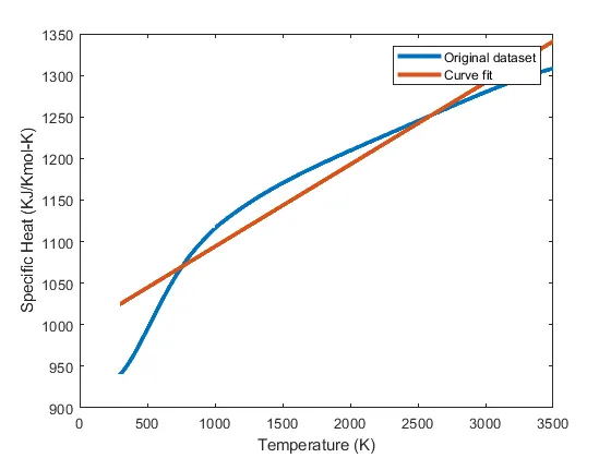
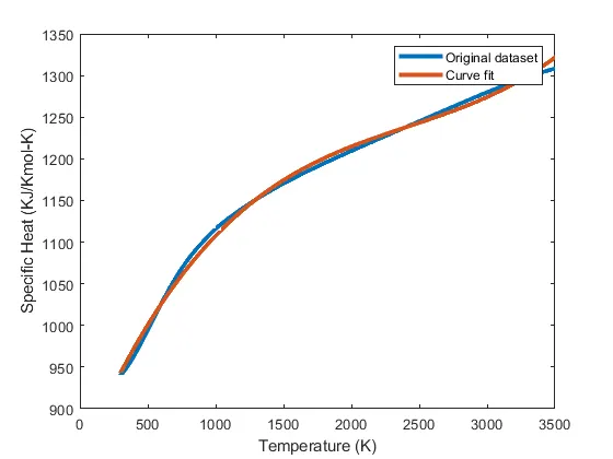
The output for the code is obtained in the form of the following plots:

1. Linear fit:

2. Cubic fit:

Program to demonstrate splitwise curve fitting method:

1. Load the given data and assign it to an array using the ‘load’ command.
2. Separate the given data into temperature and cp from column 1 and column 2 of the given data respectively.
3. Initialize loop control variables count lower as ‘cl’ and count upper as ‘cu’ that will carry the lower and upper values of the current split in the loop.
4. Plot the original data set in green color and a broad width.
5. Create a loop that splits the given data and calculates the coefficients and predicted cp values using the ‘polyfit’ and ‘polyval’ functions. The loop is also used to plot the current values of predicted data sets.

CODE:

%MATLAB program to demonstrate splitwise curve fitting method
clear all
close all
clc

%load the given data and assign it to an array
cp_data = load('data');

%seperate the values of temperature and cp values in respective arrays
temperature = cp_data(:,1);
cp = cp_data(:,2);

%initialise count_lower and count_upper variables which will be used in the loop
    cl = 1;
    cu = 100;

%plot the original data set
plot(temperature,cp,'linewidth',5,'color','g')
    
%Create a loop that loops for 32 times since we split the curve 32 times
for i = 1:32;
    
    %assign the current split of temperature and cp data 
    temperature1 = cp_data(cl:cu,1);
    cp = cp_data(cl:cu,2);
    
    %calculate the coefficients and calculated cp for the cubic polynomial equation
    co_effs1 = polyfit(temperature1,cp,3);
    calc_cp = polyval(co_effs1,temperature1);
    
    %plot the current split of temperature and calculated cp values
    hold on
    
    plot(temperature1,calc_cp,'linewidth',2,'color','k')
    
    axis([0 4000 900 1400]);
    
    %increment all the loop control variables
    i = i + 1;
    
    cl = cl + 100;
    cu = cu + 100; 
    
    
    
end
xlabel('Temperature (K)');
ylabel('Specific Heat (KJ/Kmol-K)');
legend('original data','pridicted data')

The output for the code is obtained in the form of the following plot:

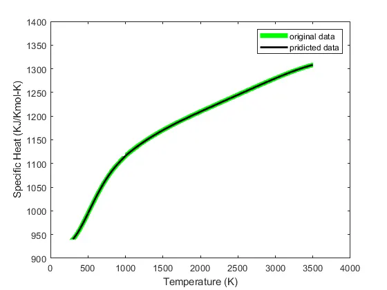
This concludes the task of programming in MATLAB to demonstrate linear and cubic curve fitting. And also, to demonstrate the splitwise method of curve fitting.

The following are the references used to learn about the project:

https://en.wikipedia.org/wiki/Curve_fitting

https://in.mathworks.com/help/matlab/ref/polyfit.html#bufp1lw-5

https://stats.stackexchange.com/questions/233414/why-are-there-large-coefficents-for-higher-order-polynomial

https://en.wikipedia.org/wiki/Runge%27s_phenomenon

https://skill-lync.com/projects/Curve-Fitting-and-criterion-to-choose-best-fit-41860