MATLAB program to solve for an ideal Otto cycle and to plot its PV diagram.

Aim: To write a MATLAB program to solve for an Ideal Otto Cycle with the following requirements,

• The program should create a PV diagram.
• The program should output the thermal efficiency of the engine.

Otto cycle: An Otto cycle is one of the Air-Standard cycles that describe the workings of a typical spark-ignition internal combustion engine. It describes a set of processes that take place while converting the chemical energy into thermal energy which is then used to achieve useful mechanical work.

The PV diagram of an ideal Otto cycle is represented as follows: (where Q₁ and Q₂ are the heat input and heat output respectively)

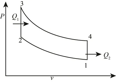
Fig 1. PV diagram of an Ideal Otto Cycle.

The processes involved in the Otto cycle is explained as follows:

Process 1 to 2:- This is the isentropic compression process during the compression stroke of the engine. Here, the charge mixture is compressed and hence, the pressure is increased, and the volume is decreased.

Process 2 to 3:- This is the constant volume heat addition process that happens when the charge is ignited with the spark. Because of the rapid chemical reaction during the combustion process, the pressure is increased at that moment while keeping a constant volume. This is also where the heat is added into the system.

Process 3 to 4:- This is the isentropic expansion process during the power stroke of the engine. Here, the rapid expansion due to the combustion process the piston travels towards the bottom dead center and hence the volume is increased, and the pressure is decreased.

Process 4 to 1:- This is the constant volume heat rejection process during the exhaust stroke to the engine. Here, the piston moves from the bottom dead center to the top dead center, and the combustion products are ejected. Hence, the pressure is decreased.

Ideal cycle vs actual cycle: The above set of processes and the PV diagram best describe an ideal Otto cycle with sharp transitions between each process. However, in reality the PV diagram of an actual Otto cycle would look something like the diagram below:

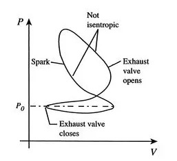
Fig 2. PV diagram of an actual Otto Cycle.

Several assumptions are made in an ideal cycle which causes the deviation from an actual cycle. Some of the assumptions made in an ideal cycle are as follows:

• The working medium is a perfect gas, obeying the ideal gas equation at all times. (PV=nRT)
• The working medium has a constant specific heat before, during and after combustion.
• Heat source and sink are considered to be external to the medium.
• The compression and expansion process is considered to be reversible and adiabatic.
• Kinetic and Potential energies are neglected.
• The operation of the engine is assumed to be frictionless.
• The combustion process is considered to be instantaneous.
• Exhaust gases are considered to eject instantaneously.
• The thermal losses through the cylinder walls are neglected.

Formulae used to determine the different state variables in the Otto Cycle:-

Before we know how to calculate the state variables, we need the following engine parameters as inputs before computing the Pressure and Volume values at different states.

The inputs are: Bore, Stroke, Connecting Rod length, Initial Pressure (P1 assumed to be 1atm or 101325 pascals), Initial Temperature after the intake stroke (T1 in kelvins), and the temperature at the end of the compression stroke (T3 in kelvins).

Now, to compute the state variables:

At state one:

Swept volume = `pi/4` x bore x stroke

Clearance volume = o

V₁ = Swept volume + Clearance volume

V₂ = Clearance volume (since the piston is at the top dead center)

At state two:

P₁V₁^γ = P₂V₂^γ (Isentropic compression process)

⇒ P₂ = P₁V₁^γ / V₂^γ

⇒ P₂ = P₁ (V₁/V₂)^γ

⇒ P₂ = P₁(compression ratio) ^γ

From ideal gas law, we have: = constant

⇒ `(P_1 V_1)/(T_1) = (P_2 V_2)/(T_2)`

⇒ `T_2=(P_2 V_2)/(P_1 V_1 ) T_1`

At state three:

State three represents the endpoint of the constant volume compression process. Hence we have,

V₃ = V₂

Again, using the ideal gas law: We have,

`(P_3 V_3)/T_3 =(P_2 V_2)/T_2`

⇒ `P_3=P_2 (T_3/T_2 )`

At state four:

State four represents the constant volume of heat rejection. Hence we have,

V₄ = V₁

_{⇒ P3V3^γ = P4V4^γ}

_⇒ P₄ = P₃ (V₃/V₄)^γ

Now that the state variables are calculated, we will have the values for the following variables that can be used as the coordinates for the PV diagram in the Otto cycle:

[V₁ V₂ V₃ V₄], [P₁ P₂ P₃ P₄]

The processes 1 to 2 and 3 to 4 cannot be connected with straight lines because the volume of the combustion chamber will not vary linearly with the crank angle. Hence we use the following expression that describes the Piston Kinematics to calculate the volume trace for a value of θ.

`V/V_c =1+1/2 (r_c-1)[R+1-cosθ⁡〖-(R^2-〖sin〗^2⁡θ )^(1/2) 〗 ]`

Where V = Volume trace,

V_c = Clearance volume(m³),

r_c = Compression ratio and

R = connecting rod length/crankpin radius, where crankpin radius = stroke/2.

The volume trace is derived from the above equation for a varying range of values of θ. And this can be used to define a separate user-defined function and the function can be called as many times as we want. In call the function twice in our program, once for the isentropic compression from process 1 to 2 and the second time at isentropic expansion from process 3 to 4.

The thermal efficiency of the engine is calculated as follows:

`η = 1 - 1/r^((γ-1) )`

The following is the user-defined function used to calculate the volume trace using the expression the describes the piston kinematics:

function [V] = engine_kinematics(bore,stroke,con_rod,cr,start_crank,end_crank)

crank_pin_radius = stroke/2;
R = con_rod/crank_pin_radius;

%Calculating swept volume and the clearance volume
v_s = (pi/4)*bore*stroke;
v_c = v_s/(cr-1);

theta = linspace(start_crank,end_crank,180);

%Seperating the piston kinematics expression into 3 terms for ease of use
term1 = (cr-1)*0.5;
term2 = R+1-cosd(theta);
term3 = (R^2 - sind(theta).^2).^0.5;

%Calculating the volume trace for the range of theta value
V = (1+term1*(term2-term3)).*v_c;

end

The following is the main program that is used to plot the PV diagram of an ideal Otto cycle and calculate the thermal efficiency of the engine for the sample engine parameters.

%MATLAB program to plot the PV diagram of an ideal Otto cycle

clear all
close all
clc

%The ratio of specific heats 'gamma' value is assumed to be 1.4
gamma = 1.4;

%Input state variables: P1(pascals), T1 and T2(kelvins)
p1 = 101325;
t1 = 500;
t3 = 2300;

%Sample input engine geometric parameters
bore = 0.1;
stroke = 0.1;
cr = 12;
con_rod = 0.15;

%Calculating the state variables in State 1
swept_volume = pi/4*(bore*stroke);
clearance_volume = swept_volume/(cr-1);

v1 = swept_volume + clearance_volume;
v2 = clearance_volume;

%Calculating the state variables in State 2
%Extracting P2 from isentropic compression process expressed as P1V1^gamma = P2V2^gamma
p2 = p1*cr^gamma;

%Extracting T2 from the ideal gas law that is expressed as PV/T = constant.
t2 = (p2*v2*t1)/(p1*v1);

%Calculating the state variables in State 3:
%At the end of constant volume compression, we have the following relation
v3 = v2;

%Extracting P3 from the ideal gas law that is expressed as PV/T = constant.
p3 = p2*(t3/t2);

%Calculating the state variables at State 4
%At the end of constant volume expansion, we have the following relation
v4 = v1;

%Extracting P4 from the isentropic expansion process expressed as P3V3^gamma = P4V4^gamma 
p4 = p3*(v3/v4)^gamma;

%Calling the engine kinematics function to get the points to plot at compression
V_compression = engine_kinematics(bore,stroke,con_rod,12,180,0);
constant1 = p1*v1^gamma;
P_compression = constant1./V_compression.^gamma;

%Calling the engine kinematics function to get the points to plot at expansion
V_expansion = engine_kinematics(bore,stroke,con_rod,12,0,180);
constant2 = p3*v3^gamma;
P_expansion = constant2./V_expansion.^gamma;

%Following set of commands are used to plot the PV diagram for an ideal Otto cycle 
figure(1)

hold on

plot(v1,p1,'*','color','r');
plot(V_compression,P_compression);
plot(v2,p2,'*','color','r');
plot(v3,p3,'*','color','r');
plot(V_expansion,P_expansion);
plot(v4,p4,'*','color','r');
plot([v2 v3],[p2 p3]);
plot([v1 v4],[p1 p4]);
xlabel('Volume(m^3)')
ylabel('Pressure(N/m^2)')

grid on;

%The percentage of Thermal Efficiency is calculated as follows
thermal_efficiency = (1 - 1/(cr^(gamma - 1)))*100

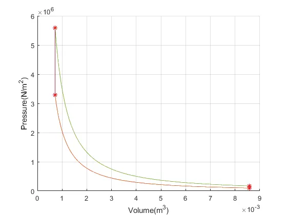
The output of the code will have the following plot and thermal efficiency value:

This concludes the project to write a program in MATLAB that

• Plots the PV diagram for an ideal Otto cycle and
• Gives the output for the thermal efficiency of an engine.