A comparison between Steady state and Transient analysis.

Aim: To compare the number of iterations taken to achieve convergence (convergence rate) between Steady-state and Transient analysis.

Objectives:

1. To pick a problem that is to be solved by both Steady-state and Transient methods.
2. Solve for the given problem in both Steady-state and Transient methods.
3. Compare the convergence rate for both the solutions.
4. Justify the numerics from the solution obtained.

Let us first look at another project that was worked upon which has a detailed description of the solution(s) to a problem that was solved in both steady-state and Transient methods. The following link will lead to that project:

https://skill-lync.com/projects/matlab-code-to-solve-for-the-2d-heat-conduction-equation-in-different-schemes

In the above shown project, it was concluded that the Successive Over Relaxation (SOR) method achieves the convergence criteria with the least number of iterations. So, the same problem definition will be taken into consideration and will be solved using the SOR method for our current comparison between Steady-state and Transient analysis.

We are considering the 2D Heat Conduction equation and solving it in both Steady-state and transient analysis. The following will be a description of the math behind the problem under consideration:

The 2D Steady-state Heat Conduction equation is as follows:

`(del^2T)/(delx^2)+(del^2T)/(dely^2)=0`

And the 2D Transient-state Heat Conduction equation is as follows:

`(∂T)/(∂t) = α((del^2T)/(delx^2))+((del^2T)/(dely^2))`

Where `alpha` is the thermal diffusivity.

The solution methodology, initial and boundary conditions are the same as the previous problem definition, whose link is attached above. The SOR method for both Steady-state and Transient analysis is described as follows:

Successive Over Relaxation method for Steady-state analysis:

The following is the equation used in an iterative manner until the error is acceptable.

`T_(i,j)=T_(old(i,j))*(1-ω)+(ω*T_(GS))`

Where TGS refers to the temperature obtained from the Gauss-Seidel equation and `omega` is the over-relaxation factor.

The MATLAB code that solves for the 2D Heat Conduction equation using the SOR method in both Steady-state and Transient methods is as follows:

%MATLAB code to compare Steady-state and Transient analysis
clear all
close all
clc

%defining the boundary
x = 1:10;
dx = abs(x(1)-x(2));
nx = length(x);
y = 1:10;
dy = abs(y(1)-y(2));
ny = length(y);

%defining the boundary conditions
t_top = 600;
t_bottom = 900;
t_left = 400;
t_right = 800;

%defining the initial conditions and the 1st guess value of temperature.
t = 300*ones(nx,ny);
t(1,:) = t_top;
t(ny,:) = t_bottom;
t(:,1) = t_left;
t(:,nx) = t_right;
t(1,1) = (t_left + t_bottom)/2;
t(1,ny) = (t_top + t_left)/2;
t(nx,ny) = (t_top + t_right)/2;
t(nx,1) = (t_right + t_bottom)/2;

%initialising the t_initial and t_old for future computation.
t_initial = t;
t_old = t;

%defining the k term for future simplification in Steady-state analysis.
k =  (dx^2*dy^2)/(2*(dx^2+dy^2));

%defining the tolerance and error values
tolerance = 1e-4;
error = 1;

%Defining the over relaxation factor.
omega = 1.2;

%Initialisising the iteration number.
iteration = 0;

%Starting the loop for SOR method for Steady-state analysis.
while error>tolerance
    
    %Starting the spatial loops
    for i = 2:(length(x)-1)
        for j = 2:(length(y)-1)
            
            term1 = (t(i-1,j)+t_old(i+1,j))/(dx^2);
            term2 = (t(i,j-1)+t_old(i,j+1))/(dy^2);
            t(i,j) = k*(term1 + term2);
            t(i,j) = t_old(i,j)*(1-omega)+(omega*t(i,j));
        end
    end
    
    %Updating the error value.
    error = max(max(abs(t_old - t)));   
    
    %Updating the t_old value.
    t_old = t;
    
    %Updating the iteration number.
    iteration = iteration + 1;
       
end

%Plotting the results for the Steady-state analysis.
figure(1)
[c,h] = contourf(x,y,t);
clabel(c,h);
colorbar
colormap(jet)
ax = gca;
ax.YDir = 'reverse';
xlabel('X Axis');
ylabel('Y Axis');
title({['Steady State - SOR method'],['Number of iterations = ',num2str(iteration)]});

%Defining the time-steps for Transient analysis.
T = 1000;
dt = 10;

%Defining the thermal diffusivity.
alpha = 1.2;

%initialising the k1 and k2 for future simplifications
k1 = alpha*(dt/(dx^2));
k2 = alpha*(dt/(dy^2));

%Initialising the error term.
error = 1;

%Starting the time-loop for the Transient analysis.
for nt = 1:1500

    %Starting the loop for SOR method for Transient analysis.
   while error > tolerance
    
       %Starting the spatial loops.
        for j = 2:(ny-1)
        
           for i = 2:(nx-1)
            
               term1 = 1/(1+(2*k1)+(2*k2));
               term2 = k1*term1;
               term3 = k2*term1;
               h = (t((i-1),j)+t_old((i+1),j));
               v = (t(i,(j-1))+t_old(i,(j+1)));
               t(i,j) =(t_initial(i,j)*term1)+(h*term2)+(v*term3);
               t(i,j) = t_old(i,j)*(1-omega)+omega*t(i,j);
            
           end
        
        end
    
        %Updating the error, t_old and iteration number.
       error = max(max(abs(t_old - t)));
       t_old = t;
       iteration = iteration + 1;
                
   end
    
   %Updating the t_initial value for the future time-steps.
   t_initial = t;
        
end

%Plotting the results for the Transient state analysis.
figure(2)
[c,h] = contourf(x,y,t);
clabel(c,h);
colorbar
colormap(jet)
set(gca,'YDIR','reverse');
xlabel('X Axis');
ylabel('Y Axis');
title({['Transient State - SOR method.'],['Number of iterations = ',num2str(iteration)]});

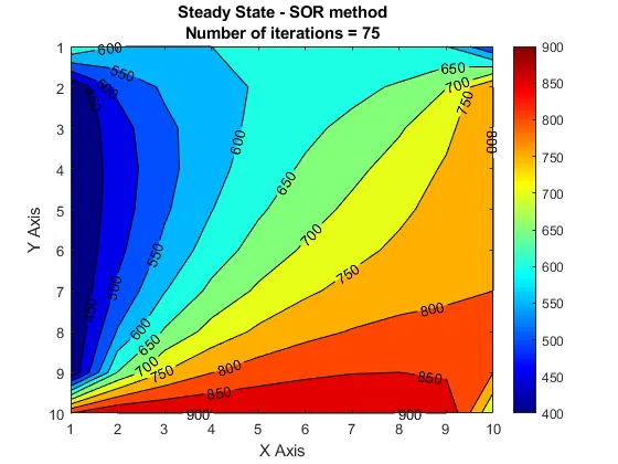
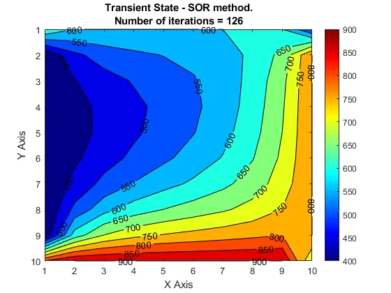
The plots obtained from the above code are as follows:

Results and discussions:

From the above plots, it is seen that the Transient analysis takes more iterations to achieve convergence than the Steady-state analysis. The reason observed for the difference in the number of iterations to achieve convergence is that the transient state analysis has an additional thermal diffusivity term and the steady-state equation is much simpler.

The very definition of the Transient analysis would mean that the rate of change in any property is not constant with respect to time. Here, the transient analysis will have to go through an additional time loop and the error is expected to at an acceptable value for each time step. This will significantly increase the computation time while solving a problem with much higher complexity.

Although in general, the Transient state analysis would give us much more practical and more precise results, it cannot be used for every problem because of the complexity involved and the increase in computation time would be much costlier to implement.