Numerical Solution for the 1D Linear Convection Equation using MATLAB.

Aim: To write a code in MATLAB that demonstrates the Numerical solution for the One-Dimensional Linear Convection Equation.

Objectives:

1. To solve for the following One-Dimensional Linear Convection Equation using Numerical Solutions:`(∂u)/(∂t)+c(∂u)/(∂x)=0`
2. The solution is to be calculated using different number of element densities.
3. Keeping the initial velocity constant, the final velocity is compared across the different number of nodes.

One-Dimensional Linear Convection Equation:

The equation under consideration for our problem is the One-Dimensional Linear Convection Equations, that is as follows:

`(∂u)/(∂t)+c(∂u)/(∂x)=0`

Using the Numerical Solution methods, the Finite Difference Method to be more specific, we will solve this equation using a time marching procedure, i.e., we will solve for the velocity at all nodes for each time-step and we will do so for all the pre-defined number of time-steps:

The initial conditions are pre-defined at time-step t0 and it is used to compute the velocity profiles for the next time step. Similarly, the further time steps are computed using the conditions of the previous time-step.

The velocity at node 2 for time-step 2 is calculated as follows:

`(∂u)/(∂t)+c(∂u)/(∂x)|_2`

⇒ `(u_2^2-u_2^1)/(Δt)+c(u_2^1-u_1^1)/(Δx)=0`

⇒ `u_2^2=u_2^1-c(Δt)/(Δx)[u_2^1-u_1^1]`

Similarly, the velocity at node 3 for time-step 3 is calculated as follows:

`(u_2^3-u_2^2)/(Δt)+c(u_2^2-u_1^2)/(Δx)=0`

⇒ `u_2^3=u_2^2-c(Δt)/(Δx)u_2^2-u_1^2`

The same can be generalised as follows for all the nodes for time-step2:

`(u_2^(n+1)-u_2^n)/(Δt)+c(u_2^n-u_1^n)/(Δx)=0`

⇒ `u_2^(n+1)=u_2^n-c(Δt)/(Δx)u_2^n-u_1^n`

In the same way we calculate the velocities at all the nodes at further time-steps. And a generalised equation for the same is as follows:

`(∂u)/(∂t)+c(∂u)/(∂x)|_T`

⇒ `(u_T^(n+1)-u_T^n)/(Δt)+c(u_T^n-u_T^n)/(Δx)=0`

⇒ `u_T^(n+1)=u_T^n-c(Δt)/(Δx)u_T^n-u_T^n`

MATLAB program to implement the above-explained method to solve for 1D linear convection equation.

The initial conditions for our code are as follows:

1. The domain length L = 1m.
2. The initial velocity profile is a step function where the velocity is equal to 2 m/s between x = 0.1 and 0.3 and 1m/s everywhere else.

Other relevant values are taken as follows:

1. Constant convection co-efficient = 1m/s.
2. Time step, dt = 0.01s
3. Simulation run time, t = 0.4s

It is to be noted that the problem is solved for 4 different element densities so they can be compared with each other.

The MATLAB code to calculate what is described above is as follows:

%MATLAB program to demonstrate 1D Linear Convection
clear all
close all
clc

%defining initial values
L = 1;
n = [21 41 81 161];
c = 1;
t = 0.4;
dt = 1e-2;
nt = t/dt;
fig = 1;

%loop for the different values for number of nodes.
for k = 1:length(n) 
    
    %defining x and dx for different values for number of nodes.
    x = linspace(0,L,n(k));
    dx = x(2) - x(1);
    
%following set of lines are used to get the node number for the step-profile for velocity in initial time-step.    
for i = 1:n(k)
    
    if(x(i) == 0.1)
       n_start = i; 
    end
    if(x(i) == 0.3)
        n_stop = i;
    end
end

%following lines are used to define the initial conditions.
u = 1*ones(1,n(k));
u(n_start:n_stop) = 2;

%following lines copy the initial velocity for future updation and reference.
u_old = u;
u_initial = u;

%loop starts for the time step integration.
for j = 1:nt  
    
%loop to calculate the velocity at each node at a given time-step.
for i = 2:n(k)
    u(i) = u_old(i) - (c*dt/dx)*(u_old(i)-u_old(i-1));
end

%updating the velocity value to be taken as a reference for the next time step.
u_old = u;

%following set of lines is used to plot the velocity profile at the given time-step.
figure(fig)

subplot(1,2,1);
plot(x,u_initial,'color','b');
grid on;
axis([0 1 0 2.1]);
xlabel('x');
ylabel('Velocity');

subplot(1,2,2);
plot(x,u,'color','b');
axis([0 1 0 2.1]);
grid on;
xlabel('x');
ylabel('Velocity');

pause(0.1);

end

fig = fig + 1;

end

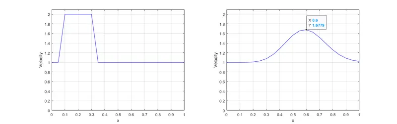
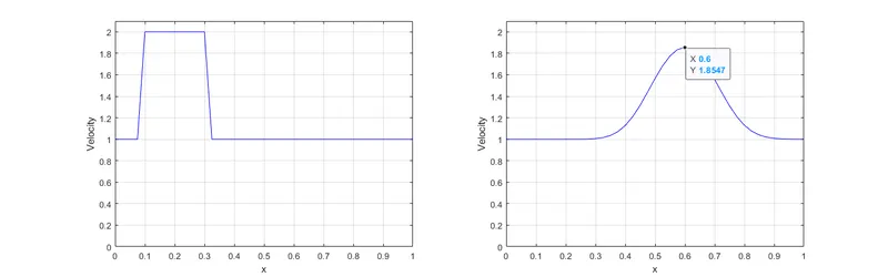
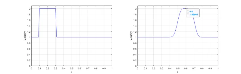
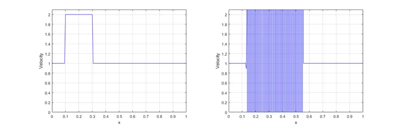
The output plots for the above program is as follows:

Conclusions:

1. From the above set of plots, we can see that the initial velocity profile gets more and more accurate as the number of nodes increase.
2. We see a general trend that the artificial diffusion in the solution is reduced as the number of nodes increase.
3. However, in the 4th plot, we can see that the solution becomes unstable and starts to oscillate. This means we can't always depend upon higher element densities to give us a more accurate solution. This method can only be taken as an introductory step in understanding the general principles and further studies regarding other methods are essential.