Understanding Stability Analysis in Linear Systems.

Aim: To solve for the given set of linear equations using iterative methods and study the convergence rate by varying Spectral Radius.

Objectives:

1. Arrange the given set of linear equations into a system of Matrices.
2. Solve the system of Matrices using Jacobi, Gauss-Seidel and SOR methods.
3. Calculate the Iteration Matrix for all the iterative methods.
4. Calculate the Eigen Value and the Spectral Radius of the Iteration Matrix.
5. Study the convergence rate by varying the Spectral Radius.

Let us now state the given set of linear equations:

`5x_1 + x_2 + 2x_3 = 10`

`-3x_1 + 9x_2 + 4x_3 = -14`

`x_1 + 2x_2 -7x_3 = 33`

Writing the above equations in the matrix form:

`[[5,1,2],[-3,9,4],[1,2,-7]] * [[x_1],[x_2],[x_3]] = [[10],[-4],[33]]`

This is in the form `AX = B`

where `A = [[5,1,2],[-3,9,4],[1,2,-7]]`

`X = [[x_1],[x_2],[x_3]]` and

`B = [[10],[-4],[33]]`

Now, we shall decompose matrix A into its Lower, Upper and Diagonal matrices.

`U = [[0,1,2],[0,0,4],[0,0,0]]`

`L = [[0,0,0],[-3,0,0],[1,2,0]]`

`D = [[5,0,0],[0,9,0],[0,0,-7]]`

Jacobi Method:

We use the following equation in a loop until convergence is achieved in order to solve for the unknowns:

`X^(n+1) = (D^-1) * (B - D^-1) * ((L + U) * x^(n))`

The following equation is used to calculate the Iteration Matrix in Jacobi Method:

`T_(iteration) = D^(-1) * (L + U)`

Gauss-Seidel Method:

We use the following equation in a loop until convergence is achieved in order to solve for the unknowns:

`X^(n+1) = (D + L)^-1 * (B - (L + D)^-1) * U * X^n`

The following equation is used to calculate the Iteration Matrix in Gauss-Seidel Method:

`T^(iteration) = (D+L)^-1 * U`

Successive Over Relaxation Method:

We use the following equation in a loop until convergence is achieved in order to solve for the unknowns:

`X^(n+1) = ((D+(omega*L)^-1))*((omega*B)-(((omega*U)-((1-omega)*D))*x^n))`

`he following equation is used to calculate the Iteration Matrix in SOR Method`

`T^(iteration) = (D + (omega*L))^-1 * ((1 - omega) * D + (omega * U))`

The following code is written in MATLAB to solve the given matrix system using the iterative methods and also to moniter the convergence rate with respect to the changing spectral radius:

%MATLAB program to solve the given matrix system using iterative solvers.
clear all
close all
clc

%Defining the decomposition of the given matrix
u = [0 1 2; 0 0 4; 0 0 0];
l = [0 0 0; -3 0 0;1 2 0];
d = [5 0 0; 0 9 0; 0 0 -7];

%Defining the coefficient matrix.
a = u + l + d;

%Defining the RHS
b = [10; -14; 33];

%Initialising the magnifaction factors
magni_fact = [0.5 1 2 3 4 5];

%Initialise the over relaxation factor to be used in SOR method.
omega = 1.2;

%Start the loop that computes the relevant data for all magnification factores.
for i = 1:length(magni_fact)
    
    %Multiply the 1st diagonal element with the magnifaction factor.
    d(1,1) = d(1,1) * magni_fact(i);
    
    %Compute the relevant fields in Jacobi Method.
    iteration_mat_jacobi = inv(d) * (l + u);
    eigen_jacobi = roots(poly(iteration_mat_jacobi));
    spectral_radius_jacobi(i) = max(real(eigen_jacobi));
    [x_jacobi,iteration_jacobi(i)] = jacobi(a,b,d);      
     
    %Compute the relevant fields in Gauss Seidel Method.
    iteration_mat_gs = inv(d + l) * u;
    eigen_gs = roots(poly(iteration_mat_gs));
    spectral_radius_gs(i) = max(real(eigen_gs));
    [x_gs,iteration_gs(i)] = gs(a,b,d);
        
    %Compute the relevant fields in SOR Method.
    iteration_mat_sor = inv(d + (omega*l)) * ((1 - omega) * d + (omega * u));
    eigen_sor = roots(poly(iteration_mat_sor));
    spectral_radius_sor(i) = max(real(eigen_sor));
    [x_sor,iteration_sor(i)] = sor(a,b,d);    
    
end

%Plotting the results.
figure(1)
subplot(2,1,1)
plot(spectral_radius_jacobi,magni_fact,'marker','o','markerface','r')
xlabel('Spectral Radius')
ylabel('Mangification Factor')
grid on;
title('Jacobi Method')
subplot(2,1,2)
plot(spectral_radius_jacobi,iteration_jacobi,'marker','o','markerface','r')
xlabel('Spectral Radius')
ylabel('Number of Iterations')
grid on;

figure(2)
subplot(2,1,1)
plot(spectral_radius_gs,magni_fact,'marker','o','markerface','r')
xlabel('Spectral Radius')
ylabel('Mangification Factor')
grid on;
title('Gauss Secidel Method')
subplot(2,1,2)
plot(spectral_radius_gs,iteration_jacobi,'marker','o','markerface','r')
xlabel('Spectral Radius')
ylabel('Number of Iterations')
grid on;

figure(3)
subplot(2,1,1)
plot(spectral_radius_sor,magni_fact,'marker','o','markerface','r')
xlabel('Spectral Radius')
ylabel('Mangification Factor')
grid on;
title('Successive Over Relaxation Method')
subplot(2,1,2)
plot(spectral_radius_sor,iteration_jacobi,'marker','o','markerface','r')
xlabel('Spectral Radius')
ylabel('Number of Iterations')
grid on;

The following is the Jacobi function:

function [x_jacobi,iteration_jacobi] = jacobi(a,b,d)

u = triu(a);
l = tril(a);

error = 1;

tolerance = 1e-4;

x_old = ones(3,1);

iteration_jacobi = 0;

while error > tolerance
    
    x_jacobi = (inv(d)) * (b - inv(d)) * ((l + u) * x_old);
    error = max(abs(x_old - x_jacobi));
    x_old = x_jacobi;
    iteration_jacobi = iteration_jacobi + 1;
    
end

end

The following is the GS function:

function [x_gs,iteration_gs] = gs(a,b,d)

u = triu(a);
l = tril(a);

error = 1;

tolerance = 1e-4;

x_old = ones(3,1);

iteration = 0;

while error > tolerance
    
    x = (inv(d + l)) * (b - inv(l + d)) * u * x_old;
    error = max(abs(x_old - x));
    x_old = x;
    iteration = iteration + 1;
    
end

x_gs = x;
iteration_gs = iteration;

end

The following is the SOR function:

function [x_sor,iteration_sor] = sor(a,b,d)

u = triu(a);
l = tril(a);

error = 1;

tolerance = 1e-4;

x_old = ones(3,1);

omega = 1.2;

iteration = 0;

while error > tolerance
    
    x = (inv(d+(omega*l)))*((omega*b)-(((omega*u)-((1-omega)*d))*x_old));
    error = max(abs(x_old - x));
    x_old = x;
    iteration = iteration + 1;
    
end

x_sor = x;
iteration_sor = iteration;

end

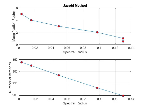
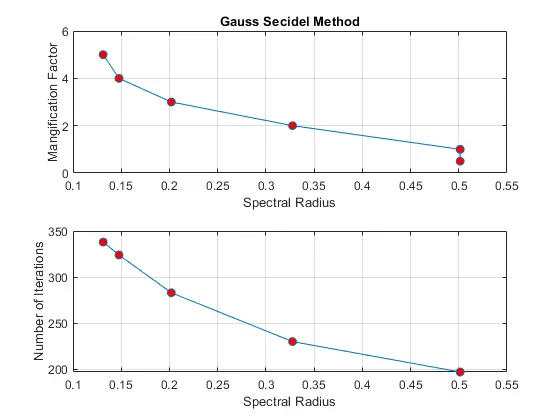
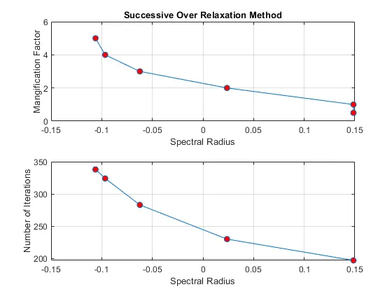
The following are the plots obtained as the output for our code:

Results ans Observations:

1. When the values for diagonal terms are larger, the values spectral radius becomes shorter.
2. When the values for the spectral radius is smaller, the number of iterations to achieve convergences is higher.