Solving for a 2nd order derivative using 4th order approximations using the Taylor Table method.
Aim: To write a code in MATLAB to get the 4th order approximation of the 2nd order derivative of the given function.
Objectives:
- To derive the 4th order approximation of the 2nd order derivative for the function:
`f(x)=e^xcos x`
- The 2nd order derivative for the given function is to be found using central difference, Skewed right-sided difference and Skewed left-sided difference.
- The errors of the respective derivative with respect to the analytical solution is to be compared.
- The absolute errors of the obtained derivatives are to be plotted.
Skewed forward differencing scheme:
The number of nodes used to compute the skewed forward differencing scheme is calculated as follows:
`N=p+q`
Where N is the number of nodes,
p is the order of derivative,
q is the order of approximation.
Therefore, we have: N = 2 + 4
⇒ N = 6
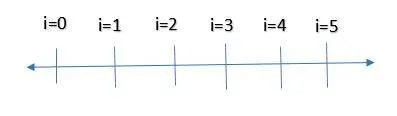
The stencil we use to compute the forward differencing looks like the following diagram:
Our hypothesis equation to calculate the 4th order approximation of the 2nd order derivative is as follows:
`dx^2(du)/(dx^2)=af(i)+bf(i+1)+cf(i+2)+df(i+3)+ef(i+4)+gf(i+5)`
We can use the following Taylor table method to find the values of the coefficients a, b, c, d, e and g to solve the 2nd order derivative.
|
f(i) |
xf(i) |
x^2f(i) |
x^3f(i) |
x^4f(i) |
x^5f(i) |
|
|
af(i) |
a |
0 |
0 |
0 |
0 |
0 |
|
bf(i+1) |
b |
b |
b/2 |
b/6 |
b/24 |
b/120 |
|
cf(i+2) |
c |
2c |
4c/2 |
8c/6 |
16c/24 |
32c/120 |
|
df(i+3) |
d |
3d |
9d/2 |
27d/6 |
81d/24 |
243d/120 |
|
ef(i+4) |
e |
4e |
16e/2 |
64e/6 |
256e/24 |
1024e/120 |
|
gf(i+5) |
g |
5g |
25g/2 |
125g/6 |
625g/24 |
3125g/120 |
|
x^2f(i) |
0 |
0 |
1 |
0 |
0 |
0 |
Therefore, we get 6 equations to solve for 6 unknowns. And it can solved by arranging and solving them in a matrix form:
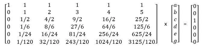
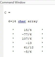
The following code was written in MATLAB to solve for the coefficients. The output was returned in the text format and the other ways of getting the coefficients was in decimals. Here, the text output is kept as a reference to solve for the derivative because the solution is more accurate with the coefficients in fractions.
clear all
close all
clc

A = [ 1 1 1 1 1 1;
      0 1 2 3 4 5;
      0 (1/2) (4/2) (9/2) (16/2) (25/2);
      0 (1/6) (8/6) (27/6) (64/6) (125/6);
      0 (1/24) (16/24) (81/24) (256/24) (625/24);
      0 (1/120) (32/120) (243/120) (1024/120) (3125/120)];

B = [0; 0; 1; 0; 0; 0];

C = rats(linsolve(A,B))
The output for the above code is as follows:
Skewed backward differencing scheme:
The number of nodes used to compute the skewed forward differencing scheme is calculated as follows:
`N=p+q`
Where, N is the number of nodes,
p is the order of derivative,
q is the order of approximation.
Therefore, we have: N = 2 + 4
⇒ N = 6
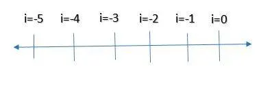
The stencil we use to compute the forward differencing looks like the following diagram:
Our hypothesis equation to calculate the 4th order approximation of the 2nd order derivative is as follows:
`dx^2(du)/(dx^2)=af(i)+bf(i-1)+cf(i-2)+df(i-3)+ef(i-4)+gf(i-5)`
We can use the following Taylor table method to find the values of the coefficients a, b, c, d, e and g to solve the 2nd order derivative.
|
f(i) |
xf(i) |
x^2f(i) |
x^3f(i) |
x^4f(i) |
x^5f(i) |
|
|
af(i) |
a |
0 |
0 |
0 |
0 |
0 |
|
bf(i+1) |
b |
-b |
b/2 |
-b/6 |
b/24 |
-b/120 |
|
cf(i+2) |
c |
-2c |
4c/2 |
-8c/6 |
16c/24 |
-32c/120 |
|
df(i+3) |
d |
-3d |
9d/2 |
-27d/6 |
81d/24 |
-243d/120 |
|
ef(i+4) |
e |
-4e |
16e/2 |
-64e/6 |
256e/24 |
-1024e/120 |
|
gf(i+5) |
g |
-5g |
25g/2 |
-125g/6 |
625g/24 |
-3125g/120 |
|
x^2f(i) |
0 |
0 |
1 |
0 |
0 |
0 |
Therefore, we get 6 equations to solve for 6 unknowns. And it can solved by arranging and solving them in a matrix form:
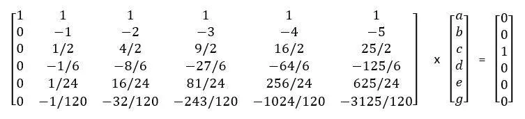
The following code was written in MATLAB to solve for the coefficients. The output was returned in the text format and the other ways of getting the coefficients were in decimals. Here too, we take the text output as a reference to solve the 2nd order derivative.
clear all
close all
clc

A = [ 1 1 1 1 1 1;
      0 -1 -2 -3 -4 -5;
      0 (1/2) (4/2) (9/2) (16/2) (25/2);
      0 -(1/6) -(8/6) -(27/6) -(64/6) -(125/6);
      0 (1/24) (16/24) (81/24) (256/24) (625/24);
      0 -(1/120) -(32/120) -(243/120) -(1024/120) -(3125/120)];

B = [0; 0; 1; 0; 0; 0];

C = rats(linsolve(A,B))
The output for the above code is as follows:
Central differencing scheme:
The number of nodes used to compute the skewed forward differencing scheme is calculated as follows:
`N=p+q-1`
Where, N is the number of nodes,
p is the order of derivative,
q is the order of approximation.
Therefore, we have: N = 2 + 4 -1
⇒ N = 5
The stencil we use to compute the forward differencing looks like the following diagram:
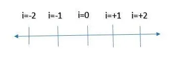
Our hypothesis equation to calculate the 4th order approximation of the 2nd order derivative is as follows:
`dx^2(du)/(dx^2)=af(i-2)+bf(i-1)+cf(i)+df(i+1)+ef(i+2)`
We can use the following Taylor table method to find the values of the coefficients a, b, c, d, e and g to solve the 2nd order derivative.
|
f(i) |
xf(i) |
x^2f(i) |
x^3f(i) |
x^4f(i) |
|
|
af(i-2) |
a |
-2a |
4a/2 |
-8a/6 |
16a/24 |
|
bf(i-1) |
b |
-b |
b/2 |
-b/6 |
b/24 |
|
cf(i) |
c |
0 |
0 |
0 |
0 |
|
df(i+1) |
d |
d |
d/2 |
d/6 |
d/24 |
|
ef(i+2) |
e |
2e |
4e/2 |
8e/6 |
16e/24 |
|
x2f(i) |
0 |
0 |
1 |
0 |
0 |
Therefore, we get 6 equations to solve for 6 unknowns. And it can solved by arranging and solving them in a matrix form:
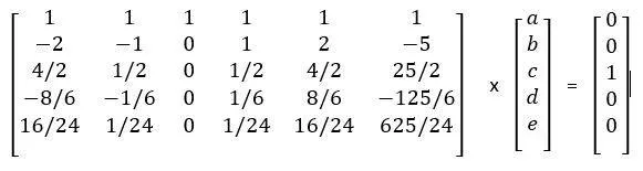
The following code was written in MATLAB to solve for the coefficients. The output was returned in the text format and the other ways of getting the coefficients were in decimals. Here too, we take the text output as a reference to solve the 2nd order derivative.
clear all
close all
clc

A = [ 1 1 1 1 1;
      -2 -1 0 1 2;
      (4/2) (1/2) 0 (1/2) (4/2);
      -(8/6) -(1/6) 0 (1/6) (8/6);
      (16/24) (1/24) 0 (1/24) (16/24)];

B = [0;0;1;0;0];

c = rats(linsolve(A,B))
The output for the above code is as follows:
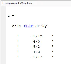
MATLAB code to solve for the 2nd order derivative of the given function and to compare the absolute errors of the different schemes is as follows:
clear all
close all
clc

%initialising the x and dx value.
x = pi/3;
dx = linspace(pi/4,pi/400,100);

%calculating the analytical derivative of the given function.
analytical_solution = -2*exp(x)*sin(x);


%For all the values of dx, we calculate the following in the for loop.
for i = 1:length(dx)

    %At first we calculate the terms in the hypothesis equation so that calculating the derivatives can be simplified later.

    a(i) = (exp(x - (5*dx(i))))*(cos(x - (5*dx(i))));

    b(i) = (exp(x - (4*dx(i))))*(cos(x - (4*dx(i))));

    c(i) = (exp(x - (3*dx(i))))*(cos(x - (3*dx(i))));

    d(i) = (exp(x - (2*dx(i))))*(cos(x - (2*dx(i))));

    e(i) = (exp(x - (dx(i))))*(cos(x - (dx(i))));

    f(i) = exp(x)*cos(x);

    g(i) = (exp(x + (dx(i))))*(cos(x + (dx(i))));

    h(i) = (exp(x + (2*dx(i))))*(cos(x + (2*dx(i))));

    j(i) = (exp(x + (3*dx(i))))*(cos(x + (3*dx(i))));

    k(i) = (exp(x + (4*dx(i))))*(cos(x + (4*dx(i))));

    l(i) = (exp(x + (5*dx(i))))*(cos(x + (5*dx(i))));

    %Calculating the derivative using skewed forward difference scheme.
    skewed_forward(i) = (((15/4)*f(i))-((77/6)*g(i))+((107/6)*h(i))-(13*j(i))+((61/12)*k(i))-((5/6)*l(i)))/(dx(i)^2);

    %Calculating the derivative using skewed backward difference scheme.
    skewed_backward(i) = (((15/4)*f(i))-((77/6)*e(i))+((107/6)*d(i))-(13*c(i))+((61/12)*b(i))-((5/6)*a(i)))/(dx(i)^2);

    %Calculating the derivative using central difference scheme.
    central_diff(i) = ((-(1/12)*d(i))+((4/3)*e(i))-((5/2)*f(i))+((4/2)*g(i))-((1/12)*h(i)))/(dx(i)^2);

    %Calculating the derivative using forward difference scheme.
    forward_diff(i) = (g(i)-f(i))/(dx(i));

    %Calculating the derivative using backward difference scheme.
    backward_diff(i) = (f(i)-e(i))/(dx(i));


    %Calculating the absolute errors of all the different schemes.
    error_central(i) = abs(central_diff(i) - analytical_solution);

    error_backward_skewed = abs(skewed_backward(i) - analytical_solution);

    error_forward_skewed = abs(skewed_forward(i) - analytical_solution);

    error_forward_diff = abs(forward_diff(i) - analytical_solution);

    error_backward_diff = abs(backward_diff(i) - analytical_solution);

end

%Plotting to compare the errors obtained in the different schemes.
figure(1)
plot(dx,error_forward_diff,'linewidth',1,'color','r','marker','o')
hold on
plot(dx,error_backward_diff,'linewidth',1,'color','b','marker','x')
xlabel('dx')
ylabel('Error value')
title('Absolute error vs dx for Forward and Backward schemes')
legend('Forward difference','Backward difference')

figure(2)

loglog(dx,error_forward_skewed,'linewidth',2,'color','g','marker','o')
hold on
loglog(dx,error_backward_skewed,'linewidth',1,'color','r','marker','x')
hold on
loglog(dx,error_central,'linewidth',1,'color','b','marker','v')
xlabel('dx')
ylabel('Error value')
title('Absolute error vs dx for various schemes')
legend('Skewed forward difference','Skewed backward difference','Central difference')
The output graphs are as follows:
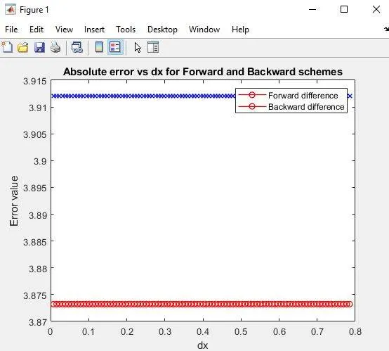
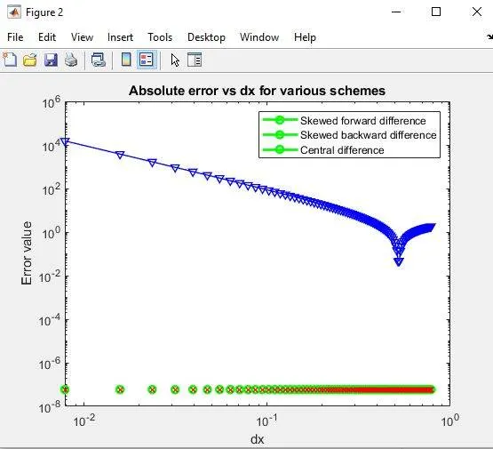
The forward and backward skewed schemes are useful in cases where the boundary nodes do not have nodes adjacent to one of the sides. In those cases, the central difference scheme cannot be used. This is the prominent advantage of the forward and backward difference schemes over the central difference scheme.