To simulate a simple pendulum by solving a second order ODE using MATLAB.

Aim: To write a program in MATLAB that simulates the motion of a simple pendulum by solving a second-order Ordinary Differential Equation.

Ordinary Differential Equations:-

Ordinary Differential Equations (ODEs) are the equations that contain derivatives of a function, and we usually try to solve for the derivatives. The derivatives represent the change of one independent variable with respect to a dependant variable.

In Engineering, ODEs are usually used to describe a transient system where an independent variable varies with respect to time. One such example for an ODE describing a transient system is that of a simple pendulum.

Simple Pendulum:-

A classic definition of a simple pendulum is one which considered to be a point mass suspended by a string or rod of negligible mass.

The point mass is first given an initial acceleration and subjected to a periodic motion to and fro from the equilibrium point at the center.

The time period for each oscillation is given by:

`T=2π√(L/g)`

Where T = time taken for one oscillation (sec),

L = length of the pendulum (m) and

g = acceleration due to gravity (m/sec²)

The acceleration of the simple pendulum is given by:

a = -g sinθ

The angle of the pendulum with respect to the equilibrium varies with time. Hence, when we try to visualize the pendulum as a line connecting two points, we can see that one end is fixed to the origin. And the coordinates for the other end can be calculated for an instantaneous value of θ. Hence, the values of the coordinates are as follows:

x0 = 0, y0 = 0,

x1 = L sinθ, y2 = -L cosθ

The value of the second coordinates varies with time. The line joining the origin and the second end can be visualized to subtend as angle θ from the equilibrium position. The rate at which θ varies with respect to time is given by the following second-order ODE:-

`(d^2 θ)/(dt^2 )+(b/m) (dθ)/dt+(g/L) sin⁡θ=0`

Where, b = damping coefficient,

m = mass (kg),

g = acceleration due to gravity (m/s²)

L = length of the pendulum (m)

In order to solve the second-order ODE, we break it down into two first-order ODEs. We first need to make the following assignments:

`θ1 = θ`,

`(dθ_1)/dt=θ_2`

When we substitute the above assignments, we get the following:

`(dθ_2)/dt+(b/m) θ_2+(g/l) sin⁡θ_1 =0`

`⇒ (dθ_2)/dt = - b/m θ_2-g/l sin⁡θ_1`

`⇒ d/dt [(θ_1;θ_2 )]=[θ_2;(- b/m) θ_2-(g/l) sin⁡θ_1 ) ]`

The objective of the project is to animate the motion of a simple pendulum by writing a program in MATLAB.

At first, we write a user-defined function that solves the second-order differential equation by breaking it down into two first-order differential equations. The function is as follows:

%User defined function to solve 2nd order ODE
function [dtheta_dt] = ode_fun(t,theta,b,g,l,m)
    theta1 = theta(1);
    theta2 = theta(2);
    dtheta1_dt = theta2;
    dtheta2_dt = -(b/m)*theta2 -(g/l)*sin(theta1);
    dtheta_dt = [dtheta1_dt;dtheta2_dt];
    
end

Now, the main function is defined with the initial conditions and then to plot for displacement and angular velocity varying with time and then to also animate the simple pendulum. The main program is as follows:

%MATLAB program to simulate pendulum motion

clear all
close all
clc

%Input variables for the test case

%Damping co-efficient is adjusted such that we get to visualize pendulum motion properly
b = 0.01;

%Acceleration due to gravity (m/s^2)
g = 9.81;

%Mass
m = 0.1;

%Length of the pendulum
l = 1;

%Initial displacement and velocity
theta_0 = [0;5];

%Time span
t_span = linspace(0,20,500);

%Solving for the 2nd order ODE
[t, results] = ode45(@(t,theta) ode_fun(t,theta,b,g,l,m),t_span,theta_0);

%Following set of commands are used to plot displacement and velocity varying with time
figure(1)
plot(t,results(:,1))
hold on
plot(t,results(:,2))
axis([0 20 -5 5])
xlabel('Plot')
ylabel('Time')

%Following set of lines is to plot for simple pendulum

%All the varying values of theta w.r.t time stored in results column 1, is assigned to a variable THETA
THETA = results(:,1);

%A counter variable is initialised to 1, it will be incremented to capture individual frames
c = 1;

%The fixed end of the pendulum is considered to be at the origin
x0 = 0;
y0 = 0;


%Using a for loop to calculate the other end of the pendulum for all angles
for i = 1:length(THETA)
    
    THETA1 = THETA(i);    
    
    x1 = l*sin(THETA1);
    %Negative sign for y because we consider the pendulum to be swinging in the 3rd and 4th quadrant
    y1 = -l*cos(THETA1);
    
    figure(2)
    
    %hold on
    plot([x0 x1],[y0 y1],'color','r', 'linewidth',2)
    hold on
    plot(x1,y1,'o','markers',20,'markerfacecolor','b')
    hold off
    grid on
    axis([-1.5 1.5 -1.5 0.5])
    pause(0.003)
    M(c) = getframe(gcf);
    c = c+1;
    
end

%Following set of commands is used to get the animation of the pendulum 
movie(M)
videofile = VideoWriter('simple_pendulum.avi','uncompressed avi');
open(videofile)
writeVideo(videofile,M)
close(videofile)

The plot for the variations of displacement and angular velocity with respect to time looks as follows:

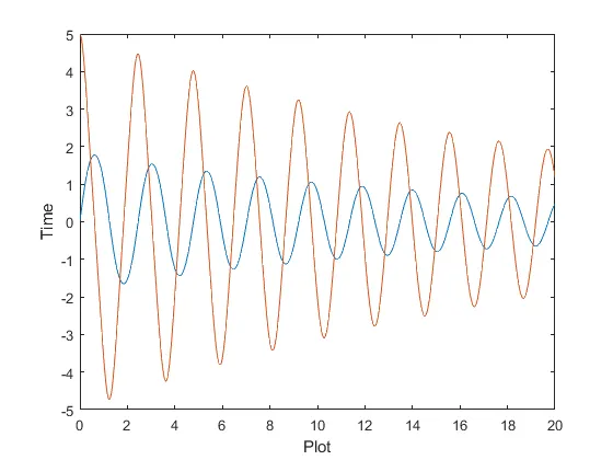
The animation of the simple pendulum is given by the following video link:

https://youtu.be/dM5SYCzLgMM

This concludes the task to write a program in MATLAB that simulates the motion of a simple pendulum by solving a second-order Ordinary Differential Equation.