Discretization basics for a range of dx.

Aim: To write a program in MATLAB that compares the first, second and fourth order approximations of the first derivative for a range of values of dx.

Objectives:

1. To write a program in MATLAB that computes the derivative of fx if fx=sin x ∕x3.
2. The first derivative is to be computed at x = pi for dx has a range of values varying from pi/40 to pi/4000 with 20 values in the range.
3. The derivative is to be calculated both numerically and analytically.
4. The numerical computation is to be done in first, second and fourth order approximations.
5. An error parameter as the absolute difference in numerical and analytical derivative at x = pi/3 is to be computed.
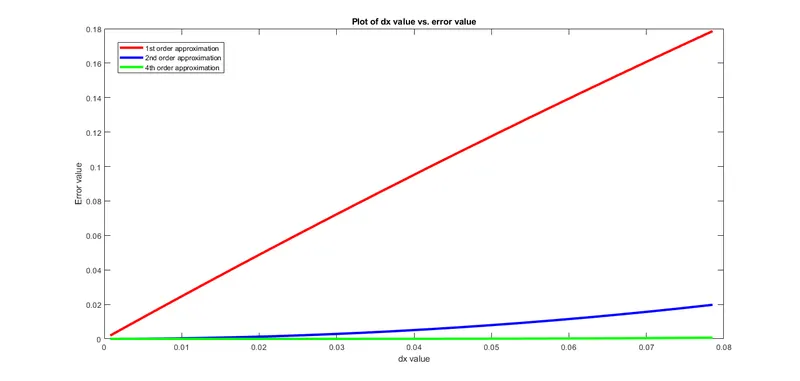
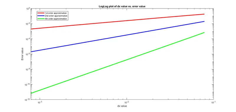
6. Graphs that helps to visualise the change in error as the value of dx decreases is to be plotted and studied.

Logic behind the program: The given function whose derivative needs to be computed is as follows:

`f(x)=sin x ∕x3`

The analytical derivative or the exact derivative is given by:

`(df)/dx=(x^3cos x -3x^2sin x)/ x^6`

We are taking the value of x as x = pi/3 and computing the derivative for the same. The result we get in from the analytical derivative will be used as the benchmark to be compared with the results we will get from computing the derivative from the first order, second order and the fourth order approximations and the error will be the absolute difference between the analytical derivative and the numerical derivative.

The numerical derivative according to the first order approximation is given as:

`(df)/dx=(f_(i+1)-f_i)/(Δx)`

The numerical derivative according to the second order approximation is given as:

`(df)/dx=(f_(i+1)-f_(i-1))/(2Δx)`

The numerical derivative according to the third order approximation is given as:

`(df)/dx=(f_(i-2)-8f_(i-1)+8f_(i+1)-f_(i+2))/(12Δx)`

The errors is calculated as follows:

Error = |numerical derivative-analytical derivative|

The MATLAB code to do the above computations is as follows:

%MATLAB program to compare numerical and analytical derivatives
clear all
close all
clc

%Initialising the values of x and dx
x = pi/3;
dx_range = linspace(pi/4000,pi/40,20);

%Computing the analytical derivative
analytic_derivative = (x^3*cos(x) - sin(x)*3*x^2)/(x^6);

for i = 1:length(dx_range)

%Computing the 1st order derivative and its error
forward_differencing(i) = ((sin(x+dx_range(i))/(x+dx_range(i))^3) - (sin(x)/x^3))/dx_range(i);
error_forward_differencing(i) = abs(analytic_derivative - forward_differencing(i));

%Computing the 2nd order derivative and its error
central_differencing(i) = ((sin(x+dx_range(i))/(x+dx_range(i))^3) - (sin(x-dx_range(i))/(x-dx_range(i))^3))/(2*dx_range(i));
error_central_differencing(i) = abs(analytic_derivative - central_differencing(i));

%Computing the 4th order derivative and its error
fourth_order_derivative(i) = (((sin(x-(2*dx_range(i))))/((x-(2*dx_range(i)))^3))-((8*sin(x-dx_range(i)))/((x-dx_range(i))^3))+((8*sin(x+dx_range(i)))/((x+dx_range(i))^3))-((sin(x+(2*dx_range(i))))/((x+(2*dx_range(i)))^3)))/(12*dx_range(i));
error_fourth_order(i) = abs(analytic_derivative - fourth_order_derivative(i));

end

%Plotting a graph to compare the error value as the dx value changes.
figure(1)
plot(dx_range,error_forward_differencing,'color','r','linewidth',3)
hold on
plot(dx_range,error_central_differencing,'color','b','linewidth',3)
hold on
plot(dx_range,error_fourth_order,'color','g','linewidth',3)
xlabel('dx value')
ylabel('Error value')
title('Plot of dx value vs. error value')
legend('1st order approximation','2nd order approximation','4th order approximation')

%Plotting a loglog plot to visualise the rate at which the error drops as the dx value is changed
figure(2)
loglog(dx_range,error_forward_differencing,'color','r','linewidth',3)
hold on
loglog(dx_range,error_central_differencing,'color','b','linewidth',3)
hold on
loglog(dx_range,error_fourth_order,'color','g','linewidth',3)
xlabel('dx value')
ylabel('Error value')
title('LogLog plot of dx value vs. error value')
legend('1st order approximation','2nd order approximation','4th order approximation')

The output graphs of the above program are as follows:

Conclusions:

1. The error values have a decreasing trend as the value of dx is lowered.
2. The error values decrease significantly as the order of approximation is increased to calculate the 1st order derivative of the given function.
3. By looking at the log-log plot, we can visualise the rate at which the error value is dropping as the value of dx is lowered.
4. The slope of the lines get steeper as the order of approximation increase, which means that in our case the slope of the 4th order approximation is the highest. Thus, the error value in the 4th order approximation drops the quickest as the value of dx is lowered.