To study the flow over a cylinder and Von Karman vortex street in Ansys Fluent.

Aim: To simulate the flow over a cylinder in Ansys Fluent and study the phenomenon of Von Karman street.

Objectives:

• To simulate the flow over the cylinder in Ansys Fluent for the case of Reynolds number equal to 100.
• To calculate the Strouhal number for the case of Reynolds number equal to 100.
• Calculate the drag and lift coefficients over a cylinder for the Reynolds numbers – 10, 100, 1000, 10000, and 100000.
• Validate the results obtained with standard literature.

The Von Karman Vortex Street is the separation of the boundary layer due to the adverse pressure gradient resulting in the reverse flow/backflow on the leeward side of a bluff body in a fluid flow reference frame. The point of separation and the frequency of separation are objects of study because these periodic disturbances generate moment on the body under consideration and hence cause vibrations.

This phenomenon occurs in a cyclic or oscillatory fashion rather than a simple acceleration. This can be observed in a wide range of natural instances such as the wind flowing around the mountains and islands, the reason why the flags flap and taut wires hum in the wind.

The study has various engineering applications such as designing a reading head in a hard drive or a DVD player that has small amplitude motion due to vortices shed from the head that limits the minimum wavelength of the laser that can be used and hence the amount of data that can be stored. This can also be studied on designing tall buildings in which the frequency of the Von Karman street does not match up with the resonant frequency of the structures.

The Reynolds number is a critical quantity that determines the periodic shedding. A flow around the cylinders shed alternating vortices in the opposite directions when the Reynolds number is between 100 to 10⁵.

The Reynolds number is defined as the ratio of the inertial forces to the viscous forces, and it is given by:

`Re=(ρvD)/ν`

Where,

`rho`--> density of the fluid flowing,

v --> fluid velocity,

D --> Diameter of the tube,

`nu`--> kinematic viscosity of the fluid.

Case setup in Ansys:

The simulation is run in a 2D scenario, which would give a top-view perspective of the flow over a cylinder. The Geometry was designed in SpaceClaim as shown below with the diameter of the cylinder as 2m, the flow region in front of the cylinder is 10 that of the diameter, i.e., 20m, and the flow region at the leeward side is 20 times the diameter of the cylinder, i.e., 40m. And the flow region above and below the cylinder is 5 times the diameter, i.e., 10m on either side.

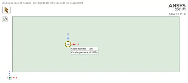
The above picture shows the geometry profile of the flow region.

The Mesh for the region is defined using the following parameters:

• All triangles method.
• Inflation layer around the cylinder with 5mm as the size of 1^st layer and total 6 layers with 1.2 as the growth.
• Face sizing: with sizing of the elements as 50mm
• Edge sizing: with the number of divisions around the cylinder as 36.

The mesh generated has 5503 nodes and 10438 elements.

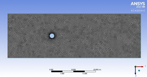
The above picture shows the generated mesh.

The names selections are as flows:

• The edge at the upwind side of the cylinder is the “inlet”.
• The edge at the leeward side of the cylinder is the “outlet”.
• The edges at above and below the cylinder are named “symmetry”.
• The edge around the cylinder is named “wall”.

The solution setup is set as follows:

• It is a pressure-based solver with absolute velocity formulation.
• The viscous model is a Laminar model.
• A “user_material” is created with the density as 1 kg/m³ and the kinematic viscosity as 0.02 kg/ms.
• The boundary condition at the inlet is velocity inlet with varying velocities for different test cases to simulate the different Reynolds numbers for each case.
• The boundary condition at the outlet is a pressure outlet with 0 gauge pressure.
• The boundary condition around the cylinder wall is set as a wall with no-slip condition.
• The boundary condition at the top and bottom side edges of the fluid domain is set as a symmetry boundary condition.
• The scheme used is SIMPLE.
• The simulation is run in a steady-state condition.

Case 1: The first case is run with conditions for Reynolds number equals 100. Hence the velocity at the inlet is 1 m/s. The solution was run for 500 iterations.

Following are the plots and results of the simulation with conditions for Reynolds number equals 100.

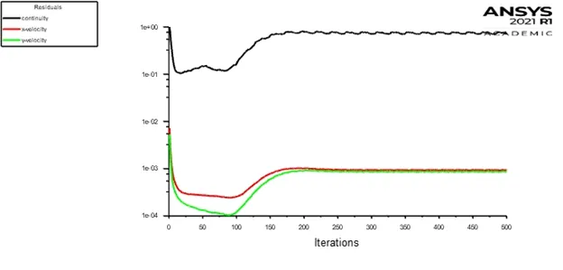
The above plot is for the scaled residuals of the through the iterations.

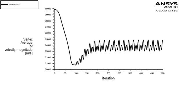
The above plot shows the variation of velocity at a probe point 8m from the center of the cylinder through the iterations.

Convergence criteria: By looking at the plots for the scaled residuals and velocity magnitude at the probe point, we can observe that the plot stabilizes at around the 200^th iteration and then the plot achieves a steady state, periodically repeating itself. Hence, we can safely conclude that the solution is converged after running for about 500 iterations.

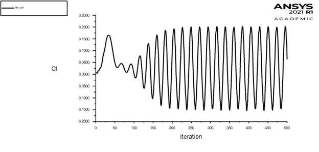
The above plot shows the variation of lift-coefficient through the iterations.

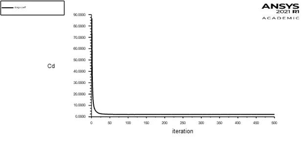
The above plot shows the variation of drag-coefficient through the iterations.

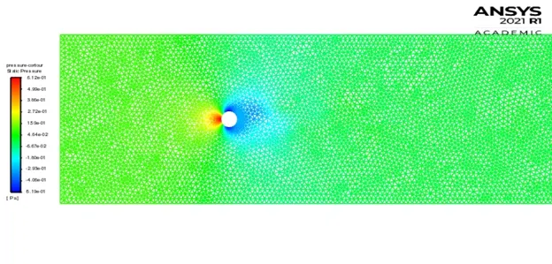
The above shows the pressure contour after 500 iterations.

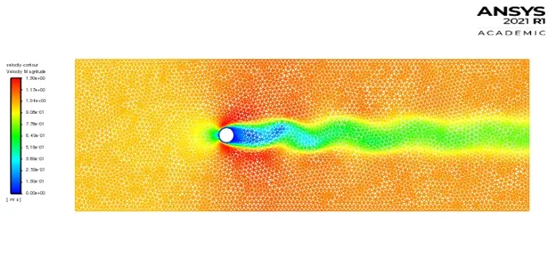
The above shows the velocity contour after 500 iterations.

The velocity contour clearly shows the vortex shedding behind the cylinder. And the pressure contour shows the low-pressure region formed at the back of the cylinder which is responsible for the backflow of the fluid that creates the periodic disturbances.

The following link will lead to the YouTube video that shows the animation generated for the test case Re = 100.

https://youtu.be/hzUPqDv2ue4

Strouhal number: The Strouhal number represents the ratio of inertial forces due to the local acceleration of the flow to the inertial forces due to the convective acceleration. Depending on the time scale of the problem, this ratio may be of order unity, and therefore its importance is not obvious. At high Strouhal numbers, oscillations dominate the flow while at low Strouhal numbers the oscillations are swept by the fast-moving fluid.

In flows characterized by a periodic motion, the Strouhal number is associated with the oscillations of the flow due to the inertial forces relative to the changes in velocity due to the convective acceleration of the flow field. Thus, an alternative definition of the Strouhal number better suited to periodic flows is given by the following expression:

`St=(fD)/U`

Where f --> frequency of the oscillations.

D --> Diameter of our cylinder.

U --> Velocity of the flow.

Since the frequency of the oscillations is one of the much-needed variables to determine the Strouhal number, it cannot be found in the case of steady-state analysis. Hence, the same settings of case 1 are used to run a transient state analysis to find the Strouhal number.

Case 2: Transient case with conditions for Re = 100.

The case was run for 2000 time steps with a time step size of 0.25 which means the simulation run was for 500 seconds. Following are the plots and results of the simulation.

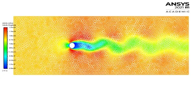
The above is the velocity contour at the end of 500 secs.

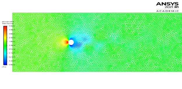
The above is the pressure contour at the end of 500 secs.

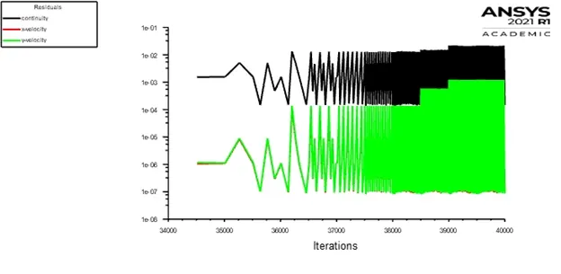
The above plot shows the variation of scale residuals over the time steps.

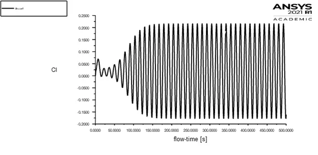
The above plot shows the variation in lift coefficient over the time steps.

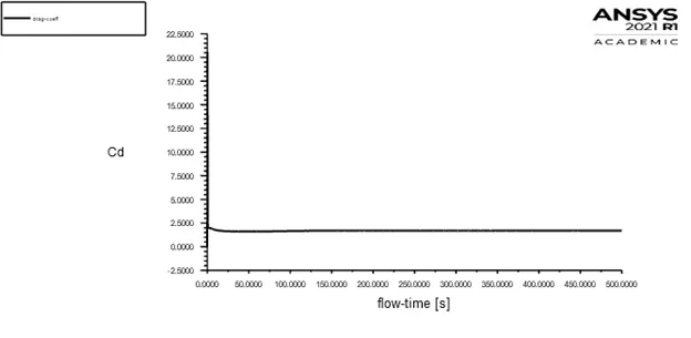
The above plot shows the variation of drag coefficient over the time steps.

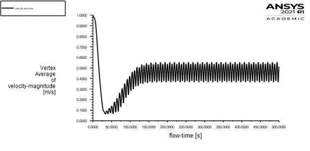
The above plot shows the variation of the velocity magnitude at the probe point over the time steps.

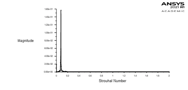
The above plot shows the variation of Strouhal number over the magnitude.

The above plot can be used to determine the Strouhal number. The file was written into an excel sheet and the corresponding Strouhal number to the maximum value of magnitude was found to be: 0.15992004. Which is very close to the reference value from the referred literature Rajani et al. [1]

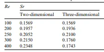
The above shows the reference value for the Strouhal number for Re = 100 from the literature.

Case 3: In case 3, we are going to be comparing the flow over the cylinder for varying Reynolds numbers. The mesh, the boundary conditions, the solutions etc are all the same as that of the Case 1, the only difference for each Reynolds number is the varying magnitude initial velocity at the inlet boundary.

Following are the different velocity inlet conditions for the corresponding Reynolds numbers.

Velocity	Reynolds number
0.1	10
1	100
10	1000
100	10000
1000	100000

The solutions were run in a steady-state solver and the following are the different plots and results obtained for the different conditions:

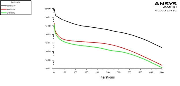
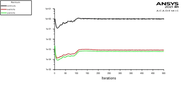
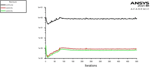
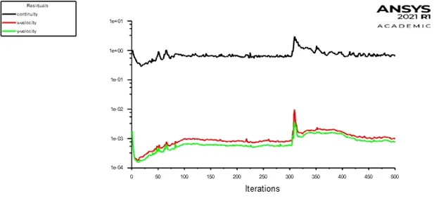
The above images show the residual plots over the iterations for varying Reynolds numbers: 10, 100, 1000, 10000, 100000.

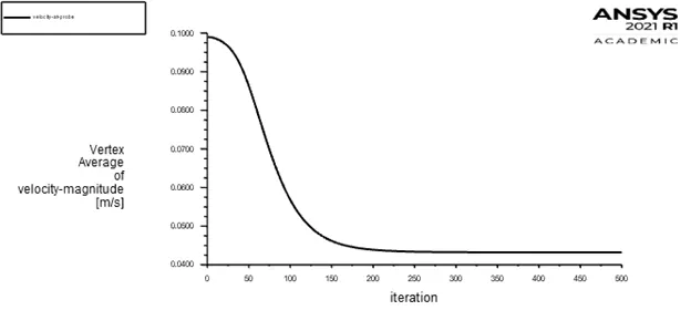
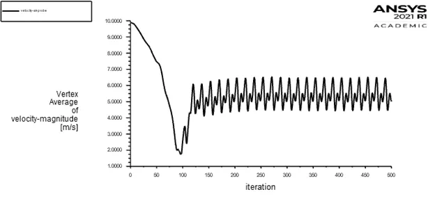
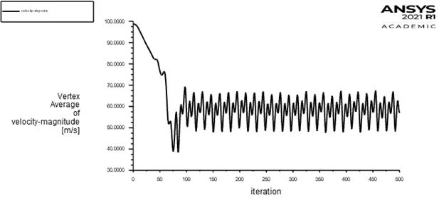
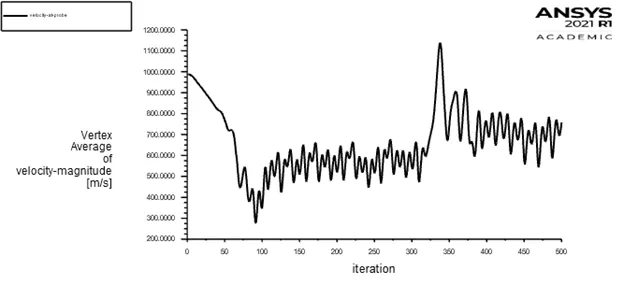
The above images show the velocity plot at the monitor point over the iterations for varying Reynolds numbers: 10, 100, 1000, 10000, 100000.

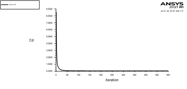
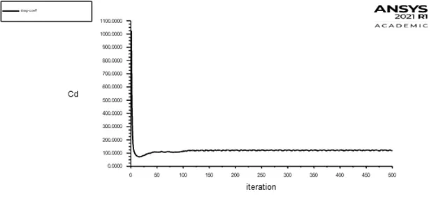
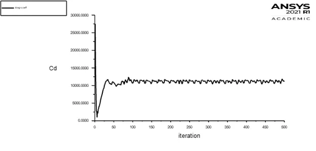
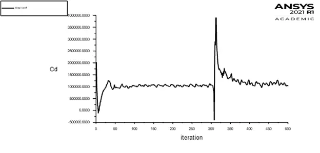
The above images show the variation in drag coefficient over the iterations for varying Reynolds numbers: 10, 100, 1000, 10000, 100000.

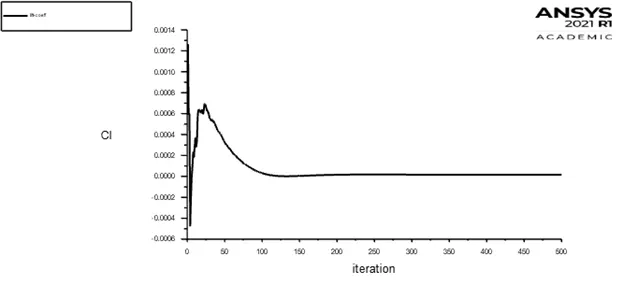
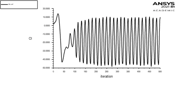
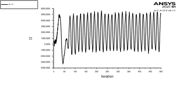
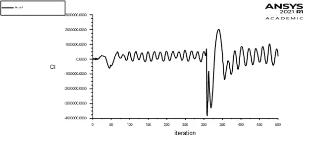
The above images show the variation in lift coefficient over the iterations for varying Reynolds numbers: 10, 100, 1000, 10000, 100000.

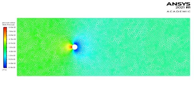
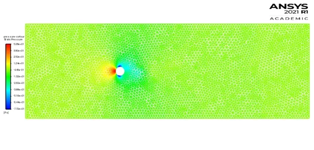
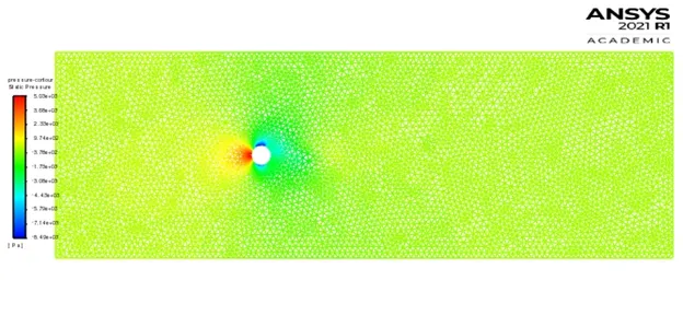
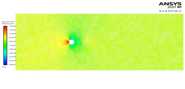
The above plot shows the pressure distribution after 500 iterations for the different Reynolds numbers: 10, 100, 1000, 10000, 100000.

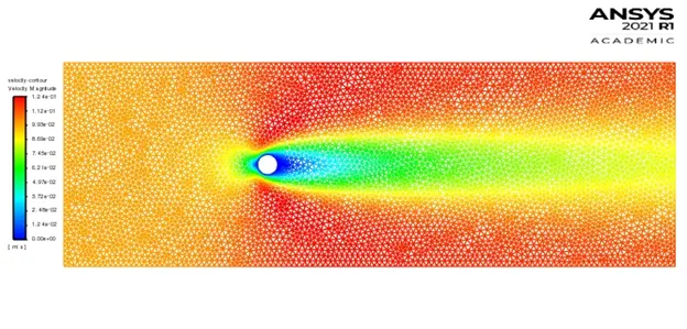
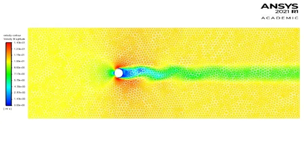
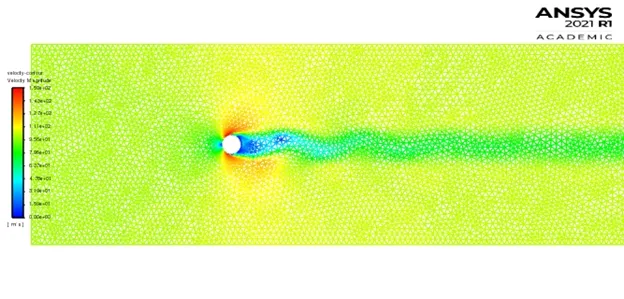
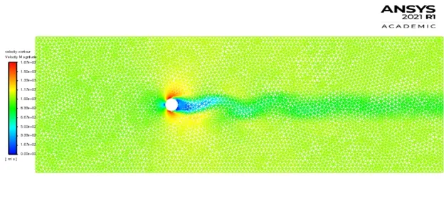
The above plot shows the velocity distribution after 500 iterations for the different Reynolds numbers: 10, 100, 1000, 10000, 100000.

Results and observations:

• As the Reynolds number increases, the frequency at which the oscillations of the vortex is seen to be increasing.
• The flow is laminar for the Reynolds numbers 10, 100, and 1000. And it can be observed in the plots for lift coefficient and the plots for the velocity at the monitor point that the flow becomes turbulent for the Reynolds number 10000 and 100000.
• We can see a clear disturbance in the cases for Reynolds numbers equal to 10000 and 100000 in the drag and lift coefficients and the velocity variation at the monitor point.

This concludes the project to study the flow over a cylinder and Von Karman Street.

Referances:

[1]https://www.sciencedirect.com/science/article/pii/S0307904X08000243