Demonstrating the Genetic Algorithm in MATLAB

Aim: To write a code in MATLAB to optimize the stalagmite function and find the global maxima of the function.

Objectives of the project:

1. To understand the concept of the Genetic Algorithm.
2. Write a MATLAB code to plot the stalagmite function.
3. Use the Genetic Algorithm to maximize the stalagmite function and study three test cases.

Genetic Algorithm:

A Genetic Algorithm is a mathematical heuristic that is inspired by the Evolution Theory by Charles Darwin. The Algorithm mimics the process of natural selection where the best individuals are selected to produce an offspring that is expected to have the best properties of both parents.

A heuristic refers to a technique that is designed to solve a problem at a much faster rate than the conventional methods of problem-solving that is too tedious.

The Genetic Algorithm is often referred to a ‘Metaheuristic’ which is a higher-level procedure designed to generate, find, or select a heuristic that “may find” a good enough solution to an optimization problem.

The Genetic Algorithm maintains a set of “population chromosomes” which are basically a set of potential solutions to the problem. The algorithm will find an optimal solution to the problem after a number of successive generations in an iterative approach. This works in a very similar way to “Natural selection”.

It is to be noted that in MATLAB, the initial population is chosen as a set of random sampling. It is then followed by further processes that hopefully results in an optimal solution to the problem.

Initial Population:

With random sampling, the chosen population is basically the potential solutions to the problem. If we are quite familiar with the problem we are working with, i.e., the function that we aim to optimize, it is best to provide lower and upper bounds to our initial random sampling. It should be a very well-educated guess, where we are absolutely sure that our solution cannot lie beyond our bounds.

Fitness function:

From the evolution theory standpoint, the fitness of any individual is nothing but the competence of that individual when compared with the others in the population. The fitness of that individual is determined by the number of desirable traits in that individual, which we would prefer to pass on to the next generation.

In our mathematical point of view, the fitness function is the one that we are trying to optimize or the one that we are looking for a solution to.

Selection:

The idea of selection is to select the fittest individuals among the population with the most desired traits and let them pass those traits to the next generation. A pair of individuals (referred to as parents) are selected based on their fitness scores and the individuals with a high fitness score is selected for the next step called reproduction/creating the next generation.

Creating the next generation:

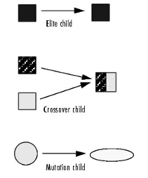
The Genetic Algorithm creates three types of children for the next generation. They are listed as follows:

1. Eliterate: are the individuals in the current generation with the best fitness scores/ the most number of desirable traits. These individuals will automatically survive to the next generation.
2. Crossover: is created by combining the vectors of a pair of parents.
3. Mutation children: are created by introducing random changes, or mutations to a single parent.

The following shows the representation of the different types of children that make it to the next generation.

Crossover:

It is the most significant phase in a Genetic Algorithm where, for each pair of parents, a crossover point is chosen at random from within the individual traits and hopefully the resulting child has an overall better set of traits when compared to the individual parents.

Mutation:

In some of the individuals of the next generation, certain traits can be subjected to a mutation with a low random probability. This mutation occurs to maintain diversity within the population and prevent premature convergence.

The stopping criteria for Genetic Algorithm:

The Algorithm uses the following criteria to determine when to stop.

1. MaxGenerations – The Algorithm runs until it reaches the maximum number or specified generations.
2. MaxTime – The Algorithm runs until it reaches the maximum specified time.
3. FitnessLimit – The Algorithm runs until the value of the fitness function for the most optimum point in the current generation is less than or equal to the FitnessLimit.
4. MaxStallGenerations – The Algorithm runs until the average relative change in the fitness function value over MaxStallGenerations is less than the function tolerance.
5. MaxStallTime – The Algorithm runs until there is no improvement in the objective function during an interval of time equal to that of MaxStallTime.
6. ConstraintTolerance – The ConstraintTolerance is not used as a stopping criterion, instead, it is used to determine the feasibility with respect to the non-linear constraints.

The Algorithm stops when any one of the above criteria is met.

Limitations of Genetic Algorithm:

1. A lot of the practical applications of the Genetic Algorithm is very difficult to implement as it would consume a lot of time. Some of the real-life problems such as structural optimizations may take several hours or even days to complete.
2. Genetic Algorithm scales exponentially with the increase in complexity such as the population size, or the number of elements exposed to mutation. This makes it very difficult to use it in complex applications such as designing an engine, a house, or a plane. Further simplification of the function to be solved to its simplest form is a necessary step to minimize complexities when scaled up. Hence, unless a very simple form of an input function is obtained, it is very difficult to find a solution to the given problem.
3. The “better” solution obtained in successive generations is only better when compared to the previous solutions. Hence, the stopping criterion is not very clear in every case.
4. There is a tendency for the Genetic Algorithm to settle for the local optimum rather than the global optimum for a given function.
5. A thorough knowledge about the problem at hand is very much essential because the solution obtained from the Genetic Algorithm cannot be taken as the absolute right solution. Hence, knowing what to expect from the solution is necessary to be able to use the Genetic Algorithm effectively.

The syntax for Genetic Algorithm in MATLAB:

The ga() function in MATLAB returns the minima of the input function using the Genetic Algorithm.

1. x = ga(fun, nvars)

This assigns the local unconstrained minimum value to x, of the unconstrained function fun. nvars is the number of design variables of fun.

2. x = ga(fun, nvars, A, b)

This assigns the local minimum value to x, of the function fun, subject to the constraints A*x ≤ b.

3. x = ga(fun, nvars, A, b, Aeq, beq)

This assigns the local minimum value to x, of the function fun, subject to the linear inequalities A*x ≤ b and Aeq*x = beq.

4. x = ga(fun, nvars, A, b, Aeq, beq, lb, ub)

This assigns the local minimum value to x, of the function fun, and defines the set of lower and upper bounds on the design variables, x, so that the solution is found in the range lb ≤ x ≤ ub.

5. x = ga(fun, nvars, A, b, Aeq, beq, lb, ub, nonlcon)

This subjects the minimization to the constraints defined in nonlcon. The function nonlcon accepts x and returns vectors C and Ceq, the nonlinear inequalities and equalities, respectively. ga minimizes the fun such that C(x) ≤ 0 and Ceq(x) = 0.

6. x = ga(fun, nvars, A, b, Aeq, beq, lb, ub, nonlcon, options)

This minimizes the default optimization parameters replaced by the values in options. We create options using optimizations.

The fitness function in our consideration:

For this project which demonstrates the Genetic Algorithm, we take the stalagmite function into consideration. Apparently, a stalagmite is a type of rock formation that grows in a specific formation under special conditions and they look like the picture below:

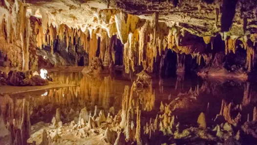
We are using a representation of the above-shown stalagmites because it contains many local minima and maxima. Hence, it will a good example to demonstrate the Genetic Algorithm to find the global optimal solution. A mathematical function to represent these stalagmites is given below.

`f(x,y)=f_(1,x) f_(1,y) f_(2,x) f_(2,y)`

where,

`f_(1,x)=[sin⁡(5.1pix+0.5) ]^6`

`f_(1,y)=[sin⁡(5.1piy+0.5) ]^6`

`f_(2,x)=exp⁡[-4 ln⁡(2) (x-0.667)^2/0.64 ]`

`f_(2,y)=exp⁡[-4 ln⁡(2) (y-0.667)^2/0.64 ]`

Our aim here in this project is to maximize the above function using a Genetic Algorithm.

Code in MATLAB to maximize the given stalagmite function:

First, we create a user defined function that returns the value for the given input array containing values for x and y. The code for the user defined function is as follows:

%A user defined function in MATLAB for the Stalagmite function

function[f]  = stalagmite(input_vector)

%Assign the values of the input array to x and y
x = input_vector(1);
y = input_vector(2);

%Function definition
fx_one = (sin((5.1*pi*x) + 0.5))^6;

fy_one = (sin((5.1*pi*y) + 0.5))^6;

fx_two = exp(-4*log(2) * (((x - 0.0667)^2)/0.64));

fy_two = exp(-4*log(2) * (((y - 0.0667)^2)/0.64));

%Return the value of f to the function call
%Using the negative sign because we're trying to 'maximise' the function using ga
f = -(fx_one * fx_two * fy_one * fy_two);

end

In the next step, we are going to be writing a code to do the following:

1. To plot the stalagmite function for each of the test studies.
2. In test case 1, we are going to use ga over 50 test runs and plot for the unbounded solutions vs test run number.
3. In test case 2, we are going to use ga over 50 test runs and plot for the bounded solutions vs test run number.
4. In test case 3, we are going to use ga over 50 test runs that uses a much higher population size than the default size and plot for the solutions vs test run number.

The code in MATLAB to do the above is given below:

The individual steps in the code are explained within the comments attached to the code:

%A MATLAB program to demonstrate Genetic Algorithm

clear all
close all
clc

%Defining the array containing values to be passed on to the stalagmite function 
x = linspace(0,0.6,150);
y = linspace(0,0.6,150);

%Creating the meshgrid over which the stalagmite function will be plotted
[xx yy] = meshgrid(x,y);

%Defining the number of test case runs for each of our case studies.
num_case = 50;

%Startin timer for the first case
tic

%Using the nested for loops, we are passing the input variables into the stalagmite function
for i = 1:length(xx)
    
    for j = 1:length(yy)
      
        input_vector(1) = xx(i,j);
        input_vector(2) = yy(i,j);
        f(i,j) = stalagmite(input_vector);
        
    end
    
end


%Getting the output the ga for each of the test runs
for i = 1:num_case
   
    [inputs,fout(i)] = ga(@stalagmite,2);
    xout(i) = inputs(1);
    yout(i) = inputs(2);
    
end

% Plotting for the stalagmite function along with the outputs for the first run
figure(1)

subplot(2,1,1)
surfc(xx,yy,-f);
hold on

%Using the shading command to hide the gridlines in the plot
%It was noticed that this also takes off a significant load on our GPU
shading interp

plot3(xout,yout,-fout,'marker','o','markerfacecolor','r');
title('Unbounded Inputs');
xlabel('x axis');
ylabel('y axis');

subplot(2,1,2)
plot(-fout);
xlabel('Iterationl');
ylabel('Function Maximum');

%Stopping the timer for the first test case
study1_time = toc

%Starting the timer for the second test run
tic

%Defining the lower and upper bounds while using ga in 2nd test run
for i = 1:num_case
   
    [inputs,fout(i)] = ga(@stalagmite,2,[],[],[],[],[0;0],[1;1]);
    xout(i) = inputs(1);
    yout(i) = inputs(2);
    
end

%Plotting for the stalagmite function along with the outputs for each test runs
figure(2)

subplot(2,1,1)
surfc(xx,yy,-f);
hold on
shading interp
plot3(xout,yout,-fout,'marker','o','markerfacecolor','r');
title('Bounded Inputs');
xlabel('x axis');
ylabel('y axis');

subplot(2,1,2)
plot(-fout);
xlabel('Iterationl');
ylabel('Function Maximum');

study2_time = toc

%Starting the timer for the 3rd test run
tic 

%Increasing the population size of the ga
options = optimoptions('ga','populationsize',200);

%Running the third test cases with the updated population size of ga
for i = 1:num_case
   
    [inputs,fout(i)] = ga(@stalagmite,2,[],[],[],[],[0;0],[1;1],[],[],options);
    xout(i) = inputs(1);
    yout(i) = inputs(2);
    
end

%Plotting for the stalagmite function along with the outputs for each test runs
figure(3)

subplot(2,1,1)
surfc(xx,yy,-f);
hold on
shading interp
plot3(xout,yout,-fout,'marker','o','markerfacecolor','r');
title('Bounded Inputs with increased population size');
xlabel('x axis');
ylabel('y axis');

subplot(2,1,2)
plot(-fout);
xlabel('Iterationl');
ylabel('Function Maximum');

study3_time = toc

The outputs obtained from the above function is discussed below:

The first case: Providing unbounded inputs to the genetic algorithm.

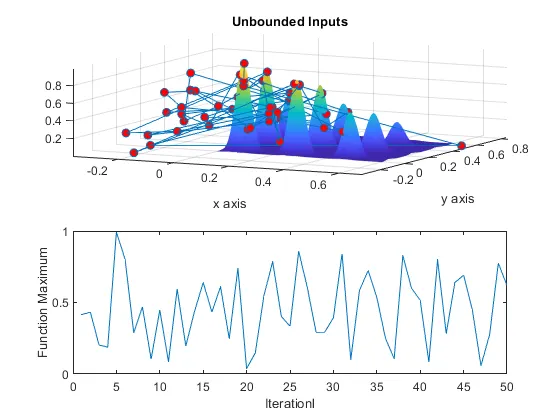
We can see that the solution for each run is all over the place. The function maxima are predicted to be at random places some of which are even outside the function definition. This is highly inaccurate.

The second test case: Providing lower and upper bounds to the inputs:

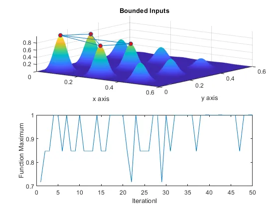
We can see that the solutions are within the function definition. But it is still not very accurate because the ga predicts the local maxima to be the global maxima in many cases.

The third test case: The population size is increased to 200 along with providing the lower and upper bounds.

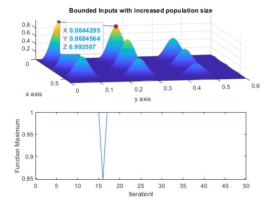
We can see that ga predicts the function maxima correctly in most of the iterations and predicts a local maxima only a negligible number of times.

However, we should note that the increase in population would result in a much significant increase in computing time. We can see the same in the study times computed within the code. The study times for each test case were computed as follows:

From the study time results, it is more than evident that with an increase in our sample space/population, the computation is significantly increased. This proves to be a major drawback to the Genetic Algorithm as more complex cases would take a much larger amount of time to compute.

This concludes the project to demonstrate the Genetic Algorithm and finding the global maxima in the given stalagmite function using MATLAB.