Demostrating file parsing in MATLAB by parsing NASA thermodynamic data.

Aim: To demonstrate file parsing for the given NASA thermodynamic data .

Objectives of the project:

1. To extract the 14 coefficients and calculate the Specific Heat, Enthalpy and Entropy for each of the species in the given data file.
2. Calculate the molecular weight of each species
3. Plot the Specific Heat, Enthalpy, and Entropy for the local temperature range (low temperature: high temperature) specific for each species.
4. Save the plots as images with appropriate names and dump them in separate folders for each species with suitable names.

Parsing: Parsing basically refers to extracting useful information from a given file by splitting the file into pieces of data that can be easily stored for further analysis/manipulation. In our project, we take the input file NASA thermodynamic data and extract useful information from it, in such a way that it can be used the study the different properties of the given species in that file.

In the given file we have sets of polynomials which NASA had come up with, that can be used to evaluate thermodynamic properties such as Specific Heat, Enthalpy, and Entropy. They have actually documented the coefficients for 1000+ species, but for the demonstration purpose, we are using the file containing the coefficients for 53 species.

The following are the formulae are used to calculate the Specific Heat, Enthalpy, and Entropy using the coefficients from the data.

Cp/R = a1 + a2 T + a3 T^3 + a4 T^3 + a5 T^4

H/RT = a1 + a2 T/2 + a3 T^2 /3 + a4 T^3 /4 + a5 T^4 /5 + a6/T

S/R = a1 lnT + a2 T + a3 T^2 /2 + a4 T^3 /3 + a5 T^4 /4 +a7

Here, it is to be noted that the FIRST 7 coefficients are HIGH- temperature coefficients and the SECOND 7 coefficients are LOW – temperature coefficients.

We have to use the local temperature ranges that are unique to each individual species and not the global temperature range.

Logic behind the MATLAB code for file parsing:

• ‘fopen’ command is used in read mode to read the given file. We must make sure that the given file which we are trying to open is in the same directory as our program.
• ‘fgetl’ command is used to read the further lines and a combination of ‘strsplit’ and ‘str2num’ is used to extract the global temperatures.
• We also skip the irrelevant lines in the given file by using the ‘fgetl’ command in a ‘for - loop’.
• The next step is to read and extract the 14 different coefficients for each of the 53 given species. Hence, we use a ‘for - loop’ that loops 53 times to read and extract the coefficients of the individual species.
• Within the data for individual species data, the headline contains information about the species name and the local temperature range. This headline is read using the ‘fgetl’ command and the species name and the local temperatures are extracted using the combination of ‘strsplit’ and ‘str2num’ commands.
• However, in order to read and extract the local temperatures, a separate logic is used. We just find the position of the letter ‘G’ in each of the headline. A simple code was written to find the position of ‘G’.

clear all
close all
clc

%Opening the data file using fopen in read mode.
data = fopen('THERMO.DAT','r');

%Skipping the 1st 5 lines using for loop.
for i = 1:5
  
  fgetl(data);
  
end

%for loop is used to print the species names and the 'G' position
for i = 1:53
  
  % Get the headline of the species using fgetl
  species = fgetl(data);
  
  %Get the 'G' position in headline using strfind
  G_pos = strfind(species,'G');
  
  %Using strsplit to extract the species name
  species = strsplit(species,' ');
  species_name = species{1};
  
  %printing the species name and 'G' position.
  %'G' position is printed twice because in some cases there are 2 Gs
  fprintf('%s %f %f n', species_name, G_pos, G_pos)
  
  %Skipping the coefficient lines using fgetl in a for loop
    for i = 1:3
  
  fgetl(data);
  
    end
end

A part of the command window showing the output of the for the above program is shown below:

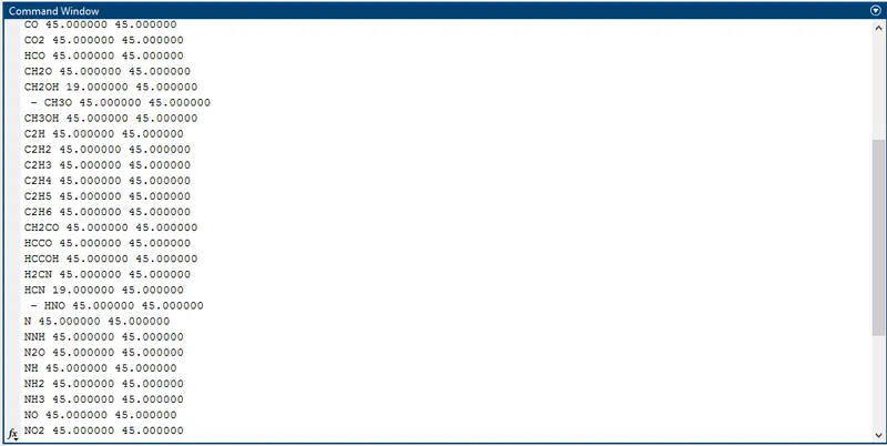
It was found that the position of ‘G’ is always at the 45^th position of the headline string. Hence, we can extract the local temperatures by taking the string from the 46^th position to the end of the headline string.

1. • The next 3 lines contain the 14 different coefficients of the given species. The 3 lines are extracted using the ‘fgetl’ command. In each of the lines, we are finding the position of ‘E’ which is the scientific notation for exponents. Each coefficient is extracted as a string with respect to the ‘E’ position in each of the lines. The coefficients in the form of a string are then converted into numbers using the ‘str2num’ command.
   • The next step is to compute the Specific Heat, Enthalpy and Entropy for each species as per its local temperature range. By default, each temperature point is true to 6 decimal places and varying them to each point would take a lot of computing time. Hence, we take only 100 divisions for temperature range to reduce the computing time.
   • A ‘for-loop’ varying between the temperature ranges is used to calculate the Specific Heat, Enthalpy, and the Entropy for each value of temperature.
   • An ‘if-else’ condition is used the segregate the lower and higher temperature coefficients and the values of Specific Heat, Enthalpy and Entropy.
   • In the next step, the graphs for temperatures vs the Specific Heat, Enthalpy and the Entropy is plotted with appropriate titles and co-ordinate labels.
   • In the next step, we have to save the plots for each species in an individual folder. Hence, we create a directory by using the ‘mkdir’ command and defining the appropriate the file path for the new file location. Then, ‘cd’ command is used open the new directory and then ‘saveas’ command is used to save the plots in a folder.
   • In the next step, we have to find the molecular weight of the individual species. The logic used to do this is as follows:
     • At first initialise the molecular weight of the species as zero, it will have an updated value in the following steps.
     • List out all the possible elements found in all the species in the given data and arrange them in an array. Then, declare another array containing the corresponding atomic mass of each element.
     • In a nested for loop that runs between the values of species names and the array containing the elements.
     • Each letter in the species name is compared with all the letters in the element array. And ‘if’ condition is used to compare with each element using ‘strcmp’ command. If the letter in the species name is the same as any letter in the element array, then the corresponding atomic mass is update (using summation) to the molecular weight of the species.
     • If the letter in the species name does not match with any of the letters in the element array, then it must be a number. In that case, the character is converted into a number using ‘str2num’ command.
     • The number is checked using an ‘if’ condition, where if the number is greater than one (we need not further use summation for molecular mass if the number is one), then the atomic mass of the previous letter is multiplied with the number minus one (because we already updated the atomic weight to the molecular weight in the nested for loops).
     • The molecular weight is printed to a separate folder using the ‘fopen’ command in write mode.
     • All the molecular weights of the 53 species are calculated in the same way within the ‘for loop’ we used to extract the coefficients and calculate their properties.

The MATLAB program for the above is as follows:

clear all
close all
clc

%Reading the given data file using fopen command
data = fopen('THERMO.DAT','r');

%Reading the 1st line that contains the global temperatures
fgetl(data);

%Following set of lines are used to extract the global temperatures
tline = fgetl(data);

global_temps = strsplit(tline, ' ');

global_low_temp = str2num(global_temps{2});
global_mid_temp = str2num(global_temps{3});
global_high_temp = str2num(global_temps{4});

%Initialising the value of the Gas constant as 8.314 (J/ mol K)
R = 8.314;

%Next 3 lines in the data file are irrelevant, hence we skip those in a for loop.
for i = 1:3
  
  fgetl(data);
  
end


%Starting a loop that extracts the coefficients, calculates Cp, H and S, plots the graphs and 
%And calculates the molecular weight of all the given 53 individual species. 
for i = 1:53
  
    %Extracting the species name and the local temperatures
  headline = fgetl(data);
  species = strsplit(headline,' ');
  species_name = species{1};
  species_temp = headline(46:end);
  
species_temp = strsplit(species_temp,' ');
local_low_temp = str2num(species_temp{2});
local_high_temp = str2num(species_temp{3});
local_mid_temp = str2num(species_temp{4});

%The 14 coefficients are listed out in three lines for each species
%Extracting the 3 lines containing the coefficients using fgetl command
first_line = fgetl(data);
second_line = fgetl(data);
third_line = fgetl(data);

%Finding the position of E in the 3 lines, which help in extracting the individual coefficients.
e_pos1 = strfind(first_line, 'E');
e_pos2 = strfind(second_line, 'E');
e_pos3 = strfind(third_line, 'E');

%The following set of lines are used to extract the 14 coefficients of each species.
char_a1 = first_line(1:(e_pos1(1)+3));
a1 = str2num(char_a1);

char_a2 = first_line((e_pos1(1)+4):(e_pos1(2)+3));
a2 = str2num(char_a2);

char_a3 = first_line((e_pos1(2)+4):(e_pos1(3)+3));
a3 = str2num(char_a3);

char_a4 = first_line((e_pos1(3)+4):(e_pos1(4)+3));
a4 = str2num(char_a4);

char_a5 = first_line((e_pos1(4)+4):(e_pos1(5)+3));
a5 = str2num(char_a5);

char_a6 = second_line(1:(e_pos2(1)+3));
a6 = str2num(char_a6);

char_a7 = second_line((e_pos2(1)+4):(e_pos2(2)+3));
a7 = str2num(char_a7);

char_a8 = second_line((e_pos2(2)+4):(e_pos2(3)+3));
a8 = str2num(char_a8);

char_a9 = second_line((e_pos2(3)+4):(e_pos2(4)+3));
a9 = str2num(char_a9);

char_a10 = second_line((e_pos2(4)+4):(e_pos2(5)+3));
a10 = str2num(char_a10);

char_a11 = third_line(1:(e_pos3(1)+3));
a11 = str2num(char_a11);

char_a12 = third_line((e_pos3(1)+4):(e_pos3(2)+3));
a12 = str2num(char_a12);

char_a13 = third_line((e_pos3(2)+4):(e_pos3(3)+3));
a13 = str2num(char_a13);

char_a14 = third_line((e_pos3(3)+4):(e_pos3(4)+3));
a14 = str2num(char_a14);

%The coefficients and the local temperatures are listed in arrays.
co_effs = [a1 a2 a3 a4 a5 a6 a7 a8 a9 a10 a11 a12 a13 a14];
temps = [local_low_temp local_mid_temp local_high_temp];
  
%100 divisions are made between low and high temperatures as a higher number takes a lot of computing time.
  T = linspace(local_low_temp,local_high_temp,100);
  
  %The values of Cp, H and S are calculated for each of the temperatures
  for j = 1:length(T)
  
      %If-else conditions are used to segregate the lower and higher temperature coefficients. 
  if T>local_mid_temp
    
    Cp = (a1 + a2.*T + a3.*T.^2 + a4.*T.^3 + a5.*T.^4).*R;
    H = (a1 + (a2.*T)./2 + (a3.*T.^2)./3 + (a4.*T.^3)./4 + (a5.*T.^4)./5 + a6./T).*T.*R;
    S = (a1.*log(T) + a2.*T + (a3.*T.^2)./2 + (a4.*T.^3)./3 + (a5.*T.^4)./4 + a7)*R;
    
  else
    
    Cp = (a8 + a9.*T + a10.*T.^2 + a11.*T.^3 + a12.*T.^4).*R;
    H = (a8 + (a9.*T)./2 + (a10.*T.^2)./3 + (a11.*T.^3)./4 + (a12.*T.^4)./5 + a13./T).*T.*R;
    S = (a8.*log(T) + a9.*T + (a10.*T.^2)./2 + (a11.*T.^3)./3 + (a12.*T.^4)./4 + a14)*R;
  end
  
  end
  
  %Following set of lines are used to plot for temperature vs Cp, H and S.
    figure(1)
    plot(T,Cp,"linewidth",3,"color",'b');
    title(species_name);
    xlabel('Temperature (K)');
    ylabel('Specific Heat [J/(mol*K)]');
    
    figure(2)
    plot(T,H,"linewidth",3,"color",'b');
    title(species_name);
    xlabel('Temperature (K)');
    ylabel('Enthalpy (J/mol)');
    
    figure(3)
    plot(T,S,"linewidth",3,"color",'b');
    title(species_name);
    xlabel('Temperature (K)');
    ylabel('Entropy [J/(mol*K)]');
    
    %Using mkdir command to open a new directory so that we can save the plots for individual plots.
    mkdir(['F:Skill-Lync filesMatlabNASA file parsingPlots', species_name]);
     
    %cd command is used to get into the directory created using mkdir.
    cd(['F:Skill-Lync filesMatlabNASA file parsingPlots', species_name]);
    
    %Following set of lines are used to save the plots generated into the created directory.
    saveas(1,'Specific Heat', 'jpg');
    saveas(2,'Enthalpy', 'jpg');
    saveas(3,'Entropy', 'jpg');
    
    %Listing out all the elements and their atomic masses, to be used in the calculation of molecular mass of each species.
    %An empty 6th element with 0 atomic mass is added to the array to prevent the error for index exceeding the array size.
    elements = ['H', 'C', 'O', 'N', 'AR',' '];
    atomic_mass = [1.008, 12.012, 15.999, 14.007, 39.948, 0];
    
    %Initialising the molecular weight as 0 before it is calculated for each species in a loop.
    molecular_weight = 0;
    
    %Following set of lines are used to calculate the molecular weight of each species.
    for a = 1:length(species_name)
       
        for b = 1:length(elements)
            
            if strcmp(species_name(a),elements(b))
                molecular_weight = molecular_weight + atomic_mass(b);
                t = b;            
            end
        
        end
    
  c = str2num(species_name(a));
  
  if c>1
      molecular_weight = molecular_weight + atomic_mass(t)*(c-1);
  end
    end
   
    %Each of the molecular weight is stored in the individual folders using the fopen command in write mode.
   molecular_mass = fopen('Molecular weight','w');
   fprintf(molecular_mass,'%s %s %s %f %s', 'The Molecular weight of ', species_name,'is', molecular_weight, 'u.');
   fclose(molecular_mass);
   
   %Following lines are used to print the molecular weight in the command window.
   molecular_mass = fopen('Molecular weight','r');
   fprintf('%s %s %s %f %s n', 'The Molecular weight of ', species_name,'is', molecular_weight, 'u.')
   
end 
   
fclose(data);

The above program creates individual folders containing plots for Temperature vs Specific Heat, Enthalpy, and Entropy for each species in the given data file.

The screenshot of the 53 folders created for each species is shown below:

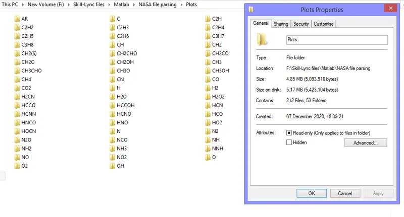
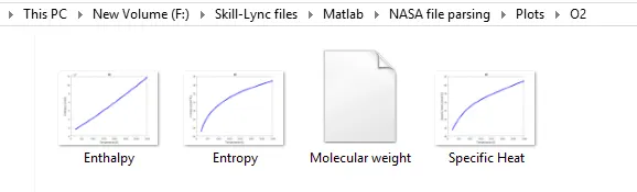
Each folder contains the plots for the graphs of Temperature vs Specific Heat, Enthalpy and Entropy. Also, it contains a file that has information about the molecular weight of the given species. The inside of a folder looks like:

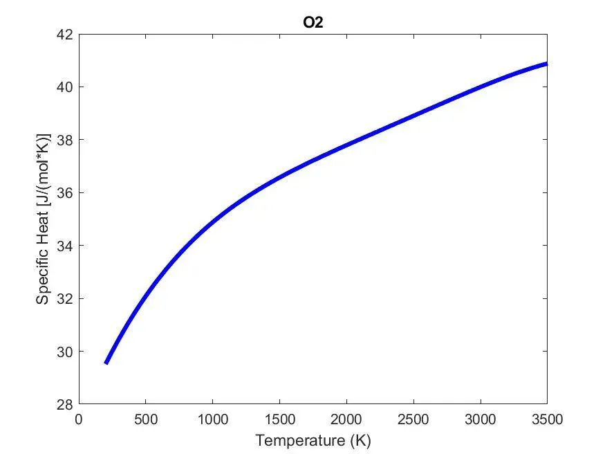
The plots for O2 are as follows:

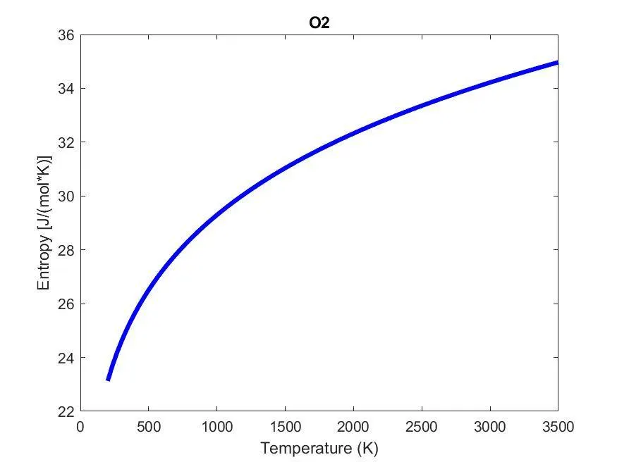
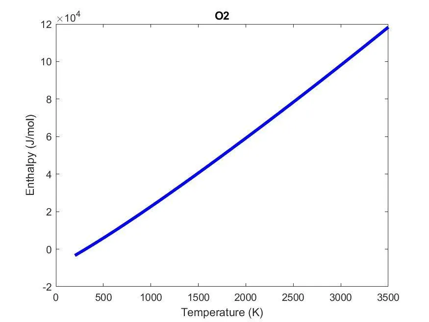
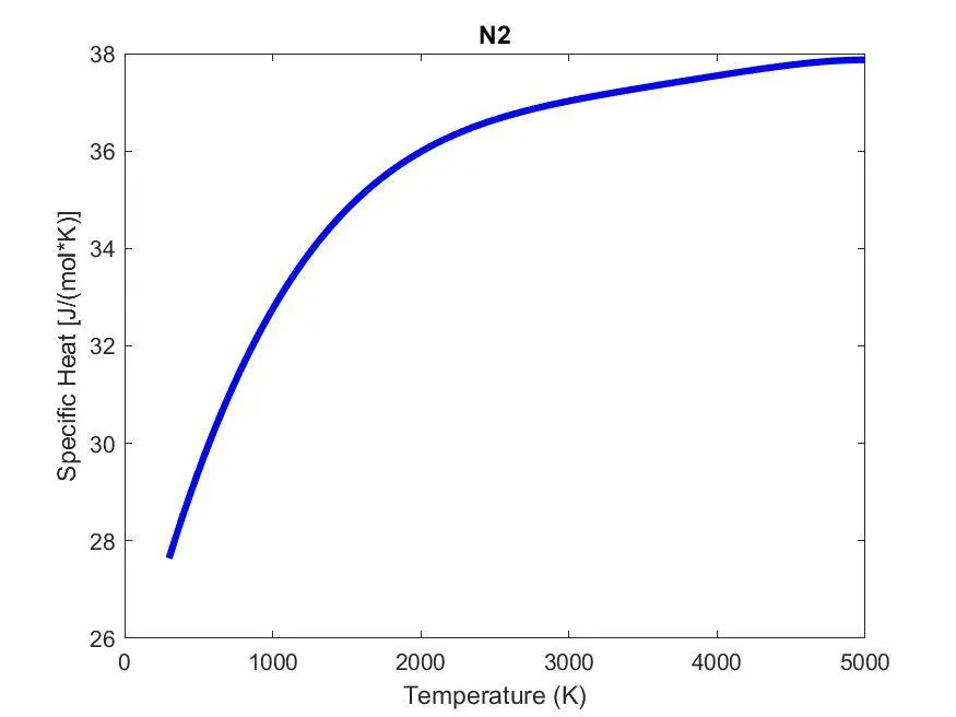
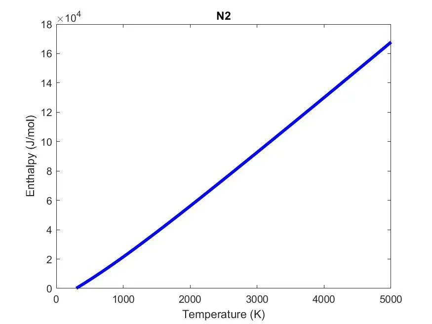
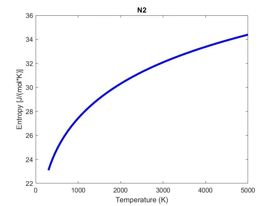
The plots for N2 are as follows:

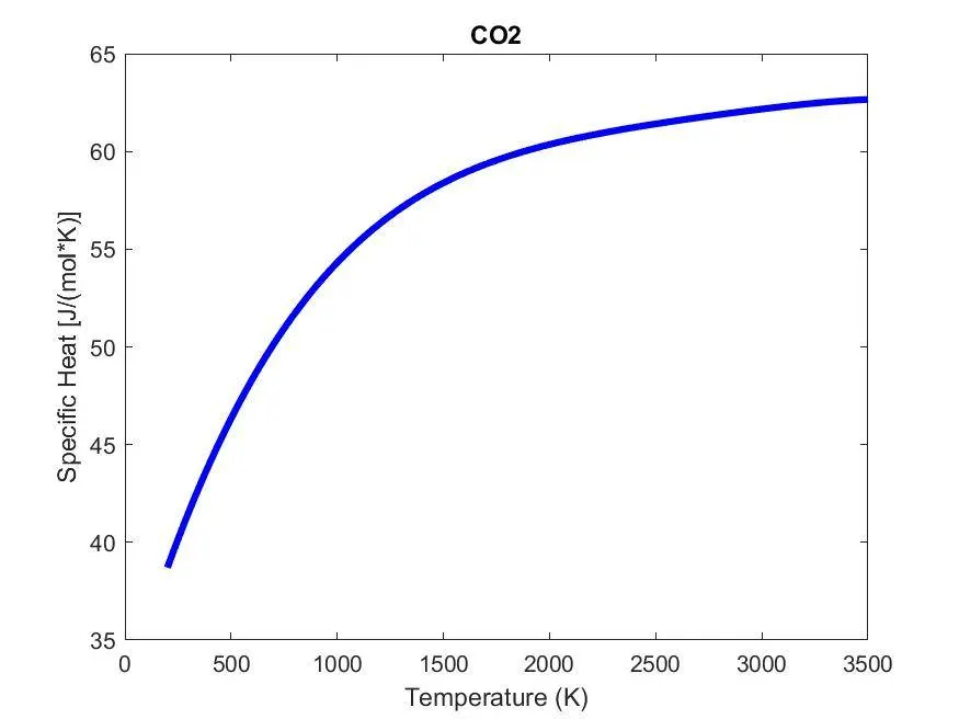
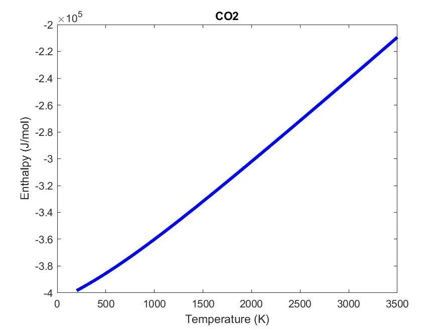
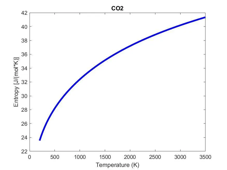
The plots for CO2 are as follows:

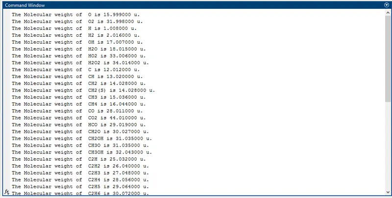
The molecular weights of each species are found and printed in each species folder. A couple of lines of code was written to print the same in the command window as well. A part of the command window that scrolls down to show the molecular weights of each species is shown as follows:

This concludes the project for demonstrating file parsing using MATLAB by parsing the NASA thermodynamic data.