Simulation of flow through a pipe in OpenFOAM using the Wedge boundary condition.
Aim: To simulate an axis-symmetric flow through a pipe in OpenFOAM using the Wedge boundary condition.
Objectives:
- To write a code in MATLAB to auto-generate a fully functional blockMeshDict file that takes inputs of pipe length, diameter and wedge angle.
- To calculate the flow variables like the hydrodynamic length of pipe, average flow velocity, max flow velocity, pressure drop, and kinematic pressure drop.
- To simulate an axis-symmetric flow through a pipe in OpenFOAM using the Wedge boundary condition and appropriate initial conditions for Pressure and Velocity.
- Obtain the plots for Velocity profile, Pressure drop profile and the Shear Stress in the Post-Processing in ParaView.
- Validate the obtained results with the analytical results.
Flow through a pipe:
Generally, the fluid flow is classified into internal or external depending on whether the fluid is forced to flow over a surface or in a conduit. Both the internal and the external flows exhibit very different characteristics. The flow under consideration is the internal flow through a pipe which is not to be confused with the open-channel flow wherein the conduit is partially filled by the fluid and thus the flow is only partially bounded by the boundaries.
Although these internal flows are very well understood on a theoretical basis, the theoretical solutions are obtained only for a few simple cases such as a fully developed laminar flow in a circular pipe. The velocity of the fluid flowing through the pipe is zero at the boundary because of the no-slip condition and it is maximum at the pipe center.
We usually calculate the average velocity of the flow Vavg which remains constant in the incompressible flow when the cross-section of the flow is constant. The flow can be categorized as laminar, transitional and turbulent depending on the Reynolds number:
`Re≤2300 ->` Laminar flow`
`2300≤Re≤4000 ->` Transitional flow,
`Re≥4000 ->`Turbulent flow.
Reynolds number is given by the equation:
`Re=(ρV_(avg) D)/μ`
Where, `rho ->` fluid density,
Vavg `->` average velocity of the fluid through the pipe,
D `->` diameter of the pipe,
`μ ->`Dynamic viscosity of the fluid.
In our case, we have the Reynolds number to be taken as 2100. By assuming the diameter of the pipe to be 2cm and the fluid to be water at 25o C, we can calculate the average velocity as following:
`V_avg=(Reμ)/(ρD)`
`μ` = 8.9X10⁻⁴ Kg/ms
`ρ` = 997.77 Kg/m3
`Vavg = (2100×(8.9×10^(-4) ))/(997.77×0.02)`
=> `Vavg = 0.093658 m/s`
The maximum velocity is given by: Umax = 2Vavg
=> Umax = 0.1873m/s
Hydrodynamic length: When we consider a fluid flow entering a circular pipe at a uniform velocity, the fluid particles in contact to the boundary surface come to a complete stop. This is because of the no-slip condition. The adjacent layers of the fluid are also slowed down because of the friction between the internal layers of the fluid. Since the overall mass flow rate of the fluid is to be conserved, the velocity of the fluid at the center is increases. This forms a velocity profile that is in a parabolic shape. And this profile becomes fully developed after a certain length of flow. This length is referred to as the Hydrodynamic length. The following diagram depicts the development of the velocity boundary layer in a pipe.
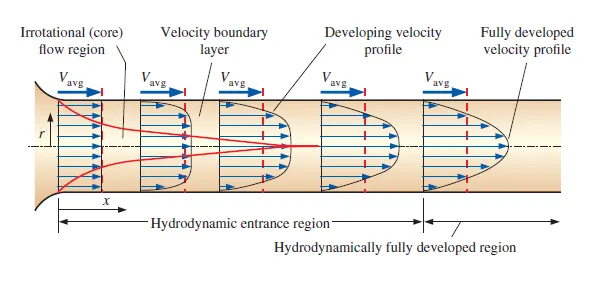
The hydrodynamic length is calculated as following:
LH = 0.05 X Re X D
=> LH = 0.05 X 2100 X 0.02 = 2.1m
For our case, let us consider the actual length of the pipe to be a little longer than the hydrodynamic length. Therefore, our overall length of the pipe will be L = 2.5m
Pressure drop and Head loss: Calculating the Pressure drops become quite important because in the pipe flow cases because these are directly correlated to the power requirements to maintain the flow. The pressure drop in a laminar flow is expressed as:
`ΔP=(32μLV_(avg))/D^2`
`=> ΔP = (32×(8.9×10^(-4) )×2.5×(0.09366))/(0.02)^2 = 16.67148 Pa`
And the kinematic pressure drop is given as:
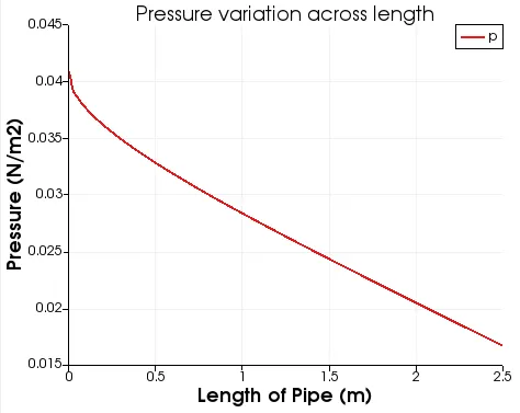
`ΔP_k=ΔP/ρ=16.67148/997.77=0.016708m`
Wedge boundary condition: The wedge boundary condition is used to define a axisymmetric conditions. The geometry and the flow should be axisymmetric along a central line such that all the physical variables of the flow have the same value and distribution at a given radius for all angles. This boundary condition is specified by two planes that must be selected on separate sides of the domain (referred to as front and back) on surfaces running along the axis. It usually works only for two-dimensional cases only.
MATLAB code to generate the blockMeshDict file:
The following code was written in MATLAB to auto-generate a fully functional blockMeshDict file that takes the inputs like pipe length, diameter and wedge angle.
clear all
close all
clc

l = 2.5;
d = 0.02;
r = d/2;
theta = 2;

f1 = fopen('blockMeshDict.txt','w');

fprintf(f1, '%sn','/*--------------------------------*- C++ -*----------------------------------*');
fprintf(f1, '%sn','  =========                 |');
fprintf(f1, '%sn','        /  F ield         | OpenFOAM: The Open Source CFD Toolbox');
fprintf(f1, '%sn','       /   O peration     | Website:  https://openfoam.org');
fprintf(f1, '%sn','      /    A nd           | Version:  8');
fprintf(f1, '%sn','     /     M anipulation  |');
fprintf(f1, '%sn','*---------------------------------------------------------------------------*/');

fprintf(f1, 'Foamfile n { n');
fprintf(f1, '%s n','    version     2.0;');
fprintf(f1, '%s n','    format      ascii;');
fprintf(f1, '%s n','    class       dictionary;');
fprintf(f1,'%s n } n','    object      blockMeshDict;');
fprintf(f1,'%s n n', '// * * * * * * * * * * * * * * * * * * * * * * * * * * * * * * * * * * * * * //');

fprintf(f1, '%s n n','convertToMeters 1;');
fprintf(f1, '%sn ( n','vertices');
fprintf(f1,'t %s n', '(0 0 0)');
fprintf(f1,'t (%d %d %d) n',0, r*cosd(theta/2), r*sind(theta/2));
fprintf(f1,'t (%d %d %d) n',0, r*cosd(theta/2), -r*sind(theta/2));
fprintf(f1,'t (%d %d %d) n',l,0,0);
fprintf(f1,'t (%d %d %d) n',l, r*cosd(theta/2), r*sind(theta/2));
fprintf(f1,'t (%d %d %d) n ); nn',l, r*cosd(theta/2), -r*sind(theta/2));

fprintf(f1,'%s n ( n','blocks');
fprintf(f1, 't %s n ); n','hex(0 3 5 2 0 3 4 1) (250 20 1) simpleGrading (1 0.1 1)');

fprintf(f1,'%s n ( n','edges')
fprintf(f1,'t %s n','arc 1 2 (0 0.01 0)');
fprintf(f1,'t %s n ); nn','arc 4 5 (2.5 0.01 0)');

fprintf(f1,'%s n ( n','boundary');

fprintf(f1,'t %s n t { n','axis')
fprintf(f1,'t t %s n','type empty;');
fprintf(f1,'t t %s n t t ( n','faces');
fprintf(f1,'t t t %s n t t ); t t t n t } n','(0 3 3 0)');

fprintf(f1,'t %s t n t { n','inlet')
fprintf(f1,'t t %s n','type patch;');
fprintf(f1,'t t %s n t t ( n','faces');
fprintf(f1,'t t t %s n t t ); t t t n t } n','(0 1 2 0)');

fprintf(f1,'t %s t n t { n','outlet')
fprintf(f1,'t t %s n','type patch;');
fprintf(f1,'t t %s n t t ( n','faces');
fprintf(f1,'t t t %s n t t ); t t t n t } n','(3 5 4 3)');

fprintf(f1,'t %s t n t { n','top')
fprintf(f1,'t t %s n','type wall;');
fprintf(f1,'t t %s n t t ( n','faces');
fprintf(f1,'t t t %s n t t ); t t t n t } n','(1 4 5 2)');

fprintf(f1,'t %s t n t { n','front')
fprintf(f1,'t t %s n','type wedge;');
fprintf(f1,'t t %s n t t ( n','faces');
fprintf(f1,'t t t %s n t t ); t t t n t } n','(0 3 4 1)');

fprintf(f1,'t %s t n t { n','back')
fprintf(f1,'t t %s n','type wedge;');
fprintf(f1,'t t %s n t t ( n','faces');
fprintf(f1,'t t t %s n t t ); t t t n t } n ); n','(0 2 5 3)');

fprintf(f1,'%s n ( n ); n','mergePatchPairs');
fprintf(f1,'%s','// ************************************************************************* //');

fclose(f1);
Following is the blockMeshDict file that was generated for the test case:
/*--------------------------------*- C++ -*----------------------------------*
  =========                 |
        /  F ield         | OpenFOAM: The Open Source CFD Toolbox
       /   O peration     | Website:  https://openfoam.org
      /    A nd           | Version:  7
     /     M anipulation  |
*---------------------------------------------------------------------------*/
FoamFile
{
    version     2.0;
    format      ascii;
    class       dictionary;
    object      blockMeshDict;
}
// * * * * * * * * * * * * * * * * * * * * * * * * * * * * * * * * * * * * * //

convertToMeters 1;

vertices
(
    (0 0 0)
    (0 0.0099985 0.00017452)
    (0 0.0099985 -0.00017452)
    (2.5 0 0)
    (2.5 0.0099985 0.00017452)
    (2.5 0.0099985 -0.00017452)
);

blocks
(
    hex (0 3 5 2 0 3 4 1) (250 20 1) simpleGrading (1 0.1 1)
);

edges
(
	arc 1 2 (0 0.01 0)
	arc 4 5 (2.5 0.01 0)
);

boundary
(
    axis
    {
        type empty;
        faces
        (
            (0 3 3 0)
        );
    }
    inlet
    {
        type patch;
        faces
        (
            (0 1 2 0)
        );
    }
    outlet
    {
        type patch;
        faces
        (
            (3 5 4 3)
        );
    }
    top
    {
    	type wall;
    	faces
    	(
    		(1 4 5 2)
    	);
    }
    front
    {
    	type wedge;
    	faces
    	(
    		(0 3 4 1)
    	);
    }
    back
    {
    	type wedge;
    	faces
    	(
    		(0 2 5 3)
    	);
    }
);

mergePatchPairs
(
);

// ************************************************************************* //
Once the mesh is created, the initial conditions for pressure and velocity need to be defined. The following is the initial conditions for velocity:
/*--------------------------------*- C++ -*----------------------------------*
  =========                 |
        /  F ield         | OpenFOAM: The Open Source CFD Toolbox
       /   O peration     | Website:  https://openfoam.org
      /    A nd           | Version:  7
     /     M anipulation  |
*---------------------------------------------------------------------------*/
FoamFile
{
    version     2.0;
    format      ascii;
    class       volVectorField;
    object      U;
}
// * * * * * * * * * * * * * * * * * * * * * * * * * * * * * * * * * * * * * //

dimensions      [0 1 -1 0 0 0 0];

internalField   uniform (0.09366 0 0);

boundaryField
{
    axis
    {
        type            empty;
    }

    inlet
    {
        type            fixedValue;
        value		 uniform (0.09366 0 0);
    }
    outlet
    {
        type            zeroGradient;
    }
    top
    {
        type            noSlip;
    }
    front
    {
        type            wedge;
    }
    back
    {
        type            wedge;
    }
}

}

// ************************************************************************* //
The following is the initial conditions for pressure:
/*--------------------------------*- C++ -*----------------------------------*
  =========                 |
        /  F ield         | OpenFOAM: The Open Source CFD Toolbox
       /   O peration     | Website:  https://openfoam.org
      /    A nd           | Version:  7
     /     M anipulation  |
*---------------------------------------------------------------------------*/
FoamFile
{
    version     2.0;
    format      ascii;
    class       volScalarField;
    object      p;
}
// * * * * * * * * * * * * * * * * * * * * * * * * * * * * * * * * * * * * * //

dimensions      [0 2 -2 0 0 0 0];

internalField   uniform 0;

boundaryField
{
    axis
    {
        type            empty;
    }

    inlet
    {
        type            zeroGradient;
    }
    outlet
    {
    	type		 fixedValue;
    	value		 uniform 0.016709;
    }
    top
    {
        type            zeroGradient;
    }
    front
    {
        type            wedge;
    }
    back
    {
        type            wedge;
    }
}

}

// ************************************************************************* //
Next is the definition of controlDict file which was set up after taking into account the average velocity and the length of pipe.
/*--------------------------------*- C++ -*----------------------------------*
  =========                 |
        /  F ield         | OpenFOAM: The Open Source CFD Toolbox
       /   O peration     | Website:  https://openfoam.org
      /    A nd           | Version:  7
     /     M anipulation  |
*---------------------------------------------------------------------------*/
FoamFile
{
    version     2.0;
    format      ascii;
    class       dictionary;
    location    "system";
    object      controlDict;
}
// * * * * * * * * * * * * * * * * * * * * * * * * * * * * * * * * * * * * * //

application     icoFoam;

startFrom       startTime;

startTime       0;

stopAt          endTime;

endTime         30;

deltaT          0.05;

writeControl    timeStep;

writeInterval	10;

purgeWrite      0;

writeFormat     ascii;

writePrecision  6;

writeCompression off;

timeFormat      general;

timePrecision   6;

runTimeModifiable true;


// ************************************************************************* //
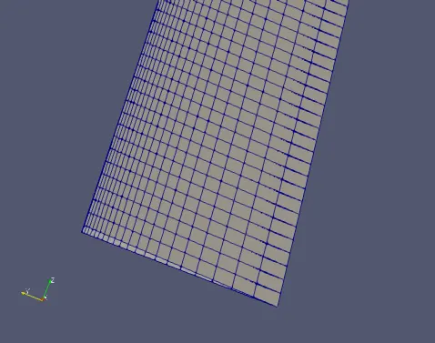
Once these files were set up, the 'blockMesh' command was used to generate the grid for our test case. The following picture shows the section oft he grid generated:
The 'icoFoam' command is used to run the solver. This specific solver was considered for the case because it is a transient solver for incompressible, laminar flow of Newtonian fluids.
Following is the velocity contour at the entrance of the pipe:
Following is the velocity contour at the fully developed region:
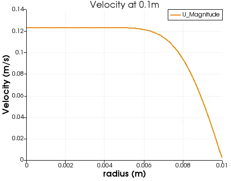
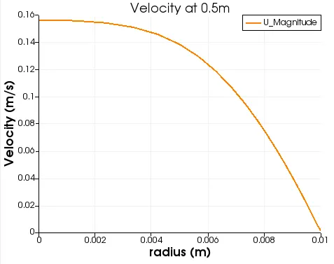
The following plot shows the velocity distribution across the radius at various lengths in the pipe:
Velocity variation at 0.1m:
Velocity variation at 0.5m:
Velocity variation at 1.5m:
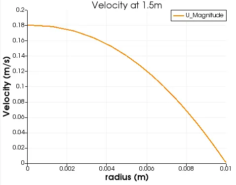
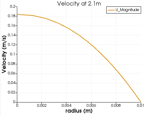
Through the above plots, we can see that the velocity profile is slowly transitioning into a parabolic shape and it is fully developed at the hydrodynamic length (2.1m).
The following plot shows the variation in Pressure across the length of the pipe:
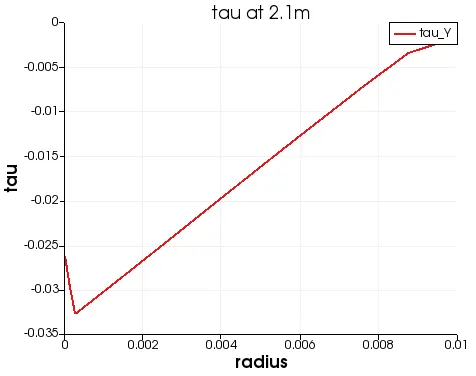
The shear stress can be calculated using the formula:
`tau = mu (du)/dy`
The following plot shows the shear stress distribution across the radius at the fully developed region (2.1m):
Comparison between analytical results and the simulation results:
| Analytical results | Simulation results | Percentage Error | |
| Max. Velocity | 0.18732 | 0.183805 | 1.88% |
| Pressure at outlet | 0.01671 | 0.01699 | 1.67% |
This concludes the project for simulating the flow in a pipe in OpenFOAM with a Wedge boundary condition.