Stability analysis in an unsteady problem.

Aim: To run a stability analysis in an unsteady state problem definition.

Objectives:

1. To choose a well-defined problem that is solved using unsteady-state methods.
2. To define the stability criteria for the given problem.
3. To demonstrate the conditions at which the solution is stable and unstable.

Problem definition:

The below link leads to the project that explains the problem under consideration and also elaborates the solution methodology at both steady and unsteady state analysis.

https://skill-lync.com/projects/matlab-code-to-solve-for-the-2d-heat-conduction-equation-in-different-schemes

Here, we are going to consider the CFL condition to describe the stability conditions for unsteady flows.

CFL stands for Courant–Friedrichs–Lewy and Culbert B. Laney’s definition of the CFL condition, from the book “Computational Gasdynamics”, is as follows: "The full numerical domain of dependence must contain the physical domain of dependence." Therefore, CFL describes the flow of information within the defined grid with each time step. And the information in a cell or element is supposed to flow only to the immediate neighbouring cells or elements. The CFL is directly proportional to the time step taken to solve the problem, hence taking lower time steps would result in a lower value for CFL and thus a more stable solution is obtained.

The CFL for the current problem under consideration is calculated as follows:

`CFL = alpha * (1/dx^2+1/dy^2)* dt`

The individual terms are predefined in the problem definition is the aforementioned project link.

The following code was written in MATLAB to analyse the stability condition in the explicit method.

%MATLAB code to solve for the transient state conduction in explicit method and analyse it's stability criteria.
clear all
close all
clc

%defining the boundary.
x = 1:10;
dx = abs(x(1)-x(2));
nx = length(x);
y = 1:10;
dy = abs(y(1)-y(2));
ny = length(y);

%defining the time steps
T = 1000;
dt = 0.1;

%defining the boundary conditions.
t_top = 600;
t_bottom = 900;
t_left = 400;
t_right = 800;

%defining the initial conditions.
t = 300*ones(nx,ny);
t(1,:) = t_top;
t(ny,:) = t_bottom;
t(:,1) = t_left;
t(:,nx) = t_right;
t(1,1) = (t_left + t_bottom)/2;
t(1,ny) = (t_top + t_left)/2;
t(nx,ny) = (t_top + t_right)/2;
t(nx,1) = (t_right + t_bottom)/2;

%initialising the t_initial and t_old for future computaions
t_initial = t;
t_old = t;

%defining the thermal diffusivity.
alpha = 1.2;

%initialising the k1 and k2 for future simplifications
k1 = alpha*(dt/(dx^2));
k2 = alpha*(dt/(dy^2));

%Calculating the CFL number
cfl = alpha*((1/dx^2)+(1/dy^2))*dt;

%initialising the iteration count.
iteration = 0;

%starting the time loop. The loop is predetermined to run for 500 time steps.
for k = 1:500
    
    %starting the spatial loops.
    for j = 2:(ny-1)
        
        for i = 2:(nx-1)
            
            %calculating the temperature at a perticular point.
            term1 = (t_old(i-1,j) - 2*t_old(i,j) + t_old(i+1,j));
            term2 = (t_old(i,j-1) - 2*t_old(i,j) + t_old(i,j+1));
            t(i,j) = t_old(i,j) + (term1*k1) + (term2*k2);
            
        end
        
    end
    
    %updating the t_old and the iteration count,
    t_old = t;
    iteration = iteration + 1;
    
    %plotting the solution at each iteration.
    [c,h] = contourf(x,y,t);
    clabel(c,h);
    colorbar
    colormap(jet)
    set(gca,'YDIR','reverse');
    xlabel('X Axis');
    ylabel('Y Axis');
    title({['2D  Heat Conduction in Transient State.'],['Number of iterations = ',num2str(iteration)],['CFL = ',num2str(cfl)]});
    pause(0.01);
    
end

The final plot obtained after running the above code is as follows:

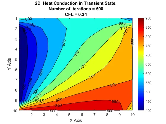
The above solution was stable and there were no observable changes in the plot after running for 500 iterations. However, in the same code, the value of dt was changed to 0.225 and the following plot was obtained after 500 iterations.

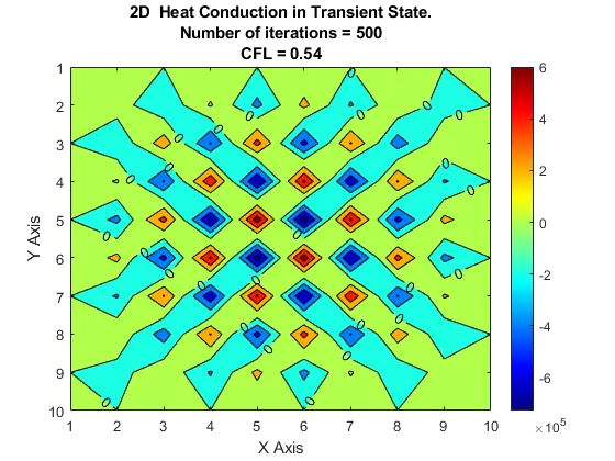
For dt = 0.225, the solution kept oscillating from start and from about 350 iterations, it started to go unstable and unrealistic temperature values are calculated at the end of 500 iterations.

The same code was again run with dt = 0.3 and the following plot is obtained.

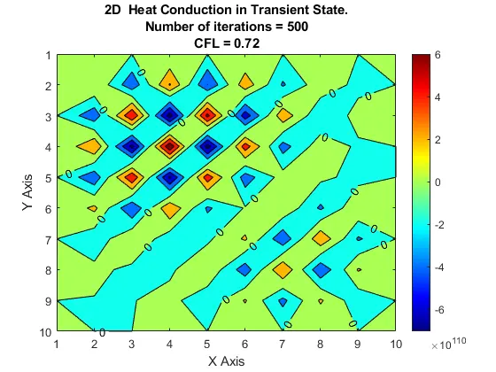
Here, the solution went unstable from the start itself and again, very unrealistic temperature conditions are obtained.

In the following three cases, we can see that higher than threshold values for CFL would take the solution to unstable conditions.

Now, the following code was written to analyse the stability with respect to CFL for the same problem definition solved using the implicit method.

clear all
close all
clc

%defining the boundary.
x = 1:10;
dx = abs(x(1)-x(2));
nx = length(x);
y = 1:10;
dy = abs(y(1)-y(2));
ny = length(y);

%defining the time steps.
T = 1000;
dt = 10;

%defining the initial conditions.
t_top = 600;
t_bottom = 900;
t_left = 400;
t_right = 800;

t = 300*ones(nx,ny);
t(1,:) = t_top;
t(ny,:) = t_bottom;
t(:,1) = t_left;
t(:,nx) = t_right;
t(1,1) = (t_left + t_bottom)/2;
t(1,ny) = (t_top + t_left)/2;
t(nx,ny) = (t_top + t_right)/2;
t(nx,1) = (t_right + t_bottom)/2;

%defining the t_initail and t_old for future computations.
t_initial = t;
t_old = t;

%defining the thermal diffusivity.
alpha = 1.2;

%initialising the k1 and k2 for future simplifications
k1 = alpha*(dt/(dx^2));
k2 = alpha*(dt/(dy^2));

%defining the tolerance and error terms for future computations.
tolerance = 1e-4;
error = 1;

%initializing the iteration count.
iteration = 0;

cfl = alpha*((1/dx^2)+(1/dy^2))*dt;

%starting the time loop.
for nt = 1:1500

    %starting the loop that runs until the error value is within tolerance.
   while error > tolerance
    
       %starting the spatial loops.
        for j = 2:(ny-1)
        
           for i = 2:(nx-1)
            
               %calculating the temperature value at a point using Jacobi method.
               term1 = 1/(1+(2*k1)+(2*k2));
               term2 = k1*term1;
               term3 = k2*term1;
               h = (t_old((i-1),j)+t_old((i+1),j));
               v = (t_old(i,(j-1))+t_old(i,(j+1)));
               t(i,j) =(t_initial(i,j)*term1)+(h*term2)+(v*term3);
            
           end
        
        end
    
        %calculating the error
       error = max(max(abs(t_old - t)));
       
       %updating the t_old and iteration count.
       t_old = t;
       iteration = iteration + 1;
                
   end
    
   %updating the t_initial.
   t_initial = t;
        
end

%plotting the solution for Jacobi method.
figure(1)
[c,h] = contourf(x,y,t);
clabel(c,h);
colorbar
colormap(jet)
set(gca,'YDIR','reverse');
xlabel('X Axis');
ylabel('Y Axis');
title({['Transient State - Implicit - Jacobi method.'],['Number of iterations = ',num2str(iteration)],['CFL = ',num2str(cfl)]});

The following plot was obtained as the result for the above code:

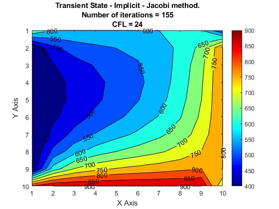
We can clearly see that both the time step that was taken and the CFL obtained are large values. But still, the solution was met with convergence criteria. This means that the stability of the solution in the implicit method is independent of the time step taken and the CFL number.

Conclusion: We can conclude that both the implicit and explicit methods have their fair share of advantages and disadvantages. The explicit methods need to meet with the stability criteria, whereas the implicit methods take more computation time. And a suitable method should be chosen to solve any problem.