Week-7 : Converting a detailed engine model to a FRM model

AIM

* To explore tutorial 9 which in details explains how to convert a existing model into a fast running model (FRM).

* To build a FRM using FRM builder approach with

bore = 102 mm

Stroke = 115 mm

Compression ratio (CR) = 17

CI engine, Twin Scroll Turbine, GT controller

INTRODUCTION

FRM is the short form of Fast running model when it comes to GT-suite models, we have run many models throughout, be it engine, afterburner or engine + afterburner, turbochargers etc, they are all detailed models. When the simulation is run for different cases in any detailed model, it will take a considerable amount of time because it is a detailed model, it will contain many components, for example if we take the intake manifold in the engine detailed model, it is modeled with a number of circular tubes, holes and flow distribution , so when the simulation is run, the flow equations (the Navier Stokes equations) have to be solved in each of these components and is therefore time consuming. To compensate for the time consumption, fast-running models are developed, in a broad sense, we can summarize it as FRM summarizes various components into a single component with simplified geometry and attributes. Taking the same intake manifold example, instead of the circular tubes, holes, and flow manifolds in the FRM, it will be a single entity or geometry called the intake manifold.

By using FRM instead of a detailed model, of course we have an advantage in simulation time, CPU time, but at the same time, the accuracy of the results will be a little compromised and the fidelity of the model will be low. The purpose of building FRM is that when testing software in the loop, hardware in the loop, etc., the real-time ECU or any software will be connected to the models, if a detailed model is used, it will be difficult to match the real-time hardware or software, so FRM will come in handy.

Examining tutorial number 9:

* The tutorial explains in detail how a high fidelity (detailed model) can be converted to FRM using the FRM conversion tool. FRM converter is a handy tool provided by GT-suite that tracks the entire conversion process.

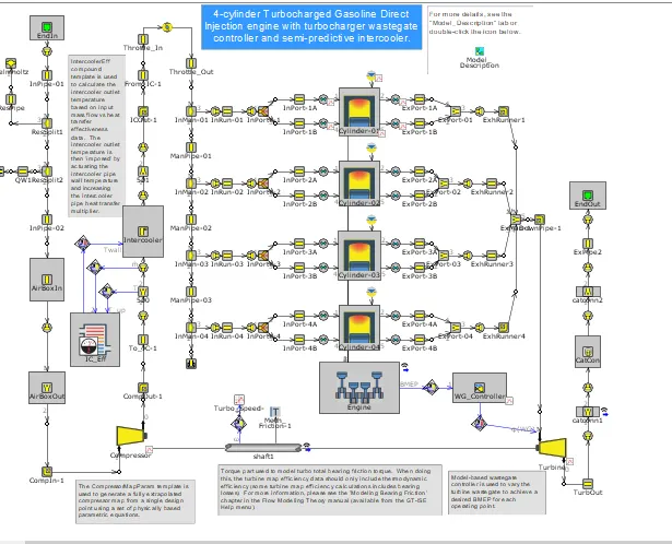
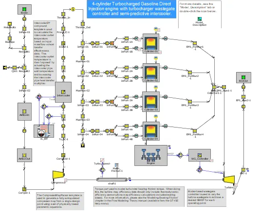
* First, we need to select the detailed model to convert it to FRM, this tutorial number 9 considers the example case SI_4Cyl_GDI_Turbo_WOT, the project map clipping of this detailed model is shown below.

* We can either convert this detailed model to FRM based on accuracy or speed, in this tutorial the simplification is done based on accuracy to compare engine performance parameters from both detailed model and FRM and determine accuracy.

* The detailed model that is opened in GT-suite is first done by FRM tagging, this option can be seen in the tools tab. Indicates all subsystems in the detailed model. We can start by simplifying the exhaust system, because the high speed flow is more at the exhaust, which affects the courant number, so the simplification starts from the exhaust pipe.

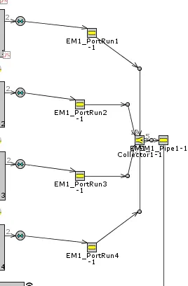
* The maximum time step limit of 1 degree of crank angle will be removed before we apply the simplification to the exhaust manifold. This is the default limit that is introduced when there is an Eng Cylinder component in the model. If the courant conditions allow a larger time step to increase the size. When the exhaust system is simplified, it looks like this:

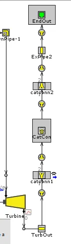
* Similar to exhaust system is exhasut from the turbine, a snip of the turbine exhaust system from detailed model is shown below,

* This system is simplified in same way as that of exhaust system of the engine. When simplified we get the exhaust from the turbine as,

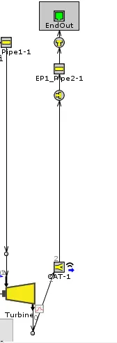
This completes the second step in conversion of detailed model to FRM and hence we have the complete project map of the second step with simplified exhaust and turbine exhaust.

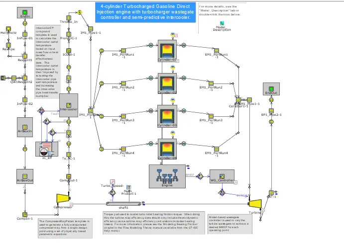
* Next is to simplify the intake manifold, the following steps are the same as for the exhaust system, minor adjustments to the attribute value of the characteristic length and expansion diameter for the combined flow need to be made.

* Characteristic length is defined as the distance traveled by a flow entering a boundary before crossing another boundary or impinging on a surface. Boundary #1 represents the boundary between IM1_pipe1-1. Fluid entering the flow manifold in this direction can pass all the way through the plenum before hitting the surface, so the characteristic length is equal to the length of the plenum.

* The other boundaries are adjacent to the runners, where the recoil from the cylinder would pass through the diameter of the chamber before hitting the chamber wall, which is why they have a characteristic length of 70mm.

* The expansion diameter defines the maximum diameter to which the flow can expand after entering the boundary. For boundary #1, this is simply the diameter of the chamber, as the fluid expands from IM1_pipe1-1 into the chamber in a straight line. Expansion diameters for other boundaries are equal to chamber diameter multiplied by 1.4. This is because as the fluid flows back into the plenum, it encounters a wider cross-section than the diameter of the plenum into which it expands. A snippet of the editing window is shown below,

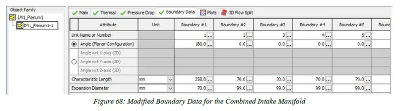
This completes the step3 of the conversion, a snip of the same is given below.

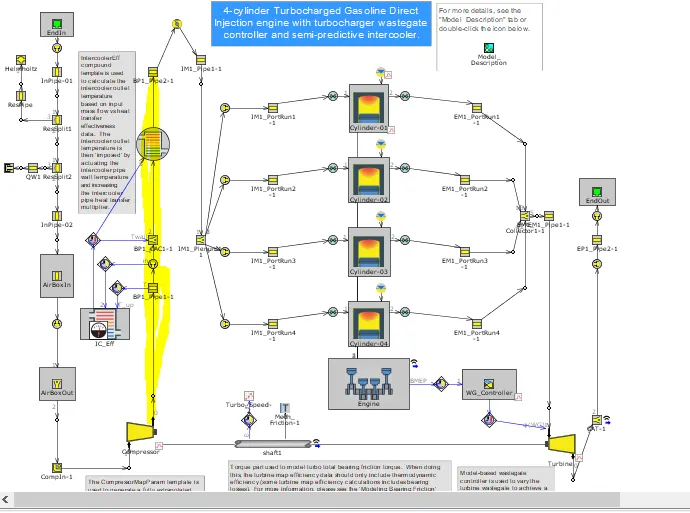
* Next is simplification of compressor outlet pipes, select boost pipes 1 from the tagged subsystem list click on simplify by accuracy. Since the intercooler core has been replaced with a flowsplit and HeatExchangerConn part. The BP1_CACC1-2 HeatExchangerConn part will be used to assure the intercooler outlet temperature is maintained.

* When the compressor coutlet pipes are simplified this completed the step4 and hence we have

* Intake pipes select intake pipes 1 from the tagged subsystem list. Click on simplify for accuracy. Collapse the FRM converter to provide space to work in the model map.This completes the simpyfing process. We have somethings like below after step5

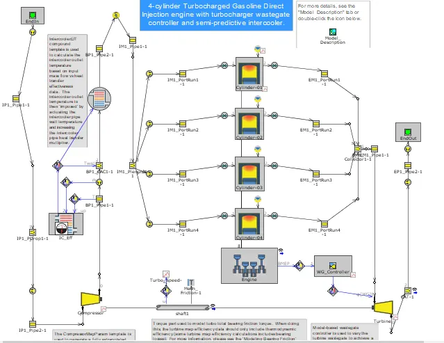
* We started with simplifying exhaust system on accuracy basis now we can further simplify the exhaust system on time step basis, by doing this we get a much simplified exhaust system as shown below,

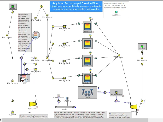
* Final step or simplifying done is cylinder slaving. By right clicking on any of the EngCylinder slaving option. For full cylinder slaving to function, each valve must be specified as either an intake or exhaust valve.

So above tutorial gives us an idea of how the existing detailed model can be converted.

* To build a FRM:

Second part of this challenge is to build a FRM with following parameters,

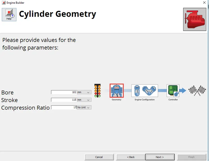
bore = 102 mm

Stroke = 115 mm

Compression ratio (CR) = 17

CI engine, Twin Scroll Turbine, GT controller.

Main purpose of building a FRM is to check how much the simulation time as well as CPU time vary, so let us first take a detailed CI model which has a turbo and a controller.

Let us consider Diesel_6Cyl_TC example case, this model has a twin turbocharger, a control unit, 6 cylinders. This example resembles much to the FRM we are building.

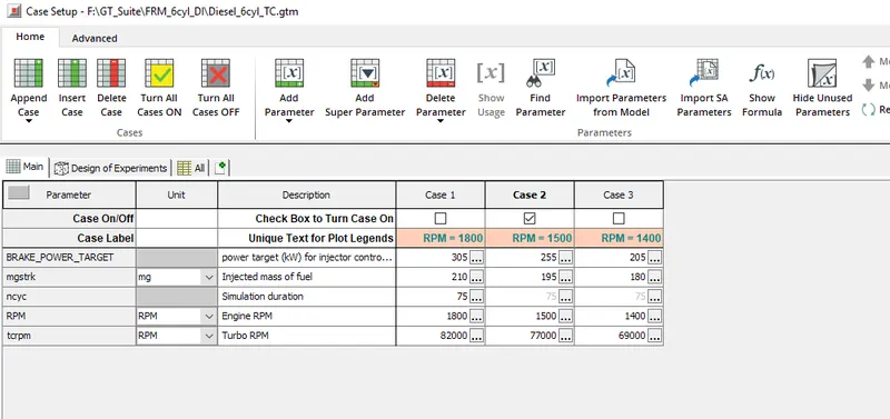
Simulation is run at engine speed = 1500 rpm, below is the snip that shows the other parameters. Even this detailed 6 cylinder engine model is set with above mentioned bore, stroke and compression ratio values.

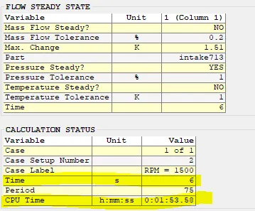
Following is the time taken for the simulation to run,

Now let us build a FRM and then run the simulaton,

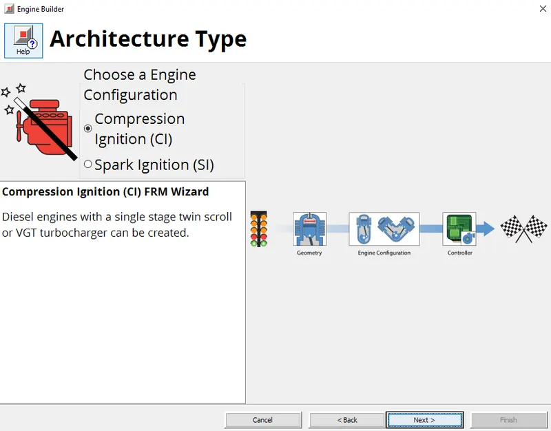
Under tools option FRM builder option is available, when we click this option we get the below window where CI engine is selected.

* When we click next we get attributes that define bore, stroke and compression ratio. Below is the snip of the window that shows the attributes defined,

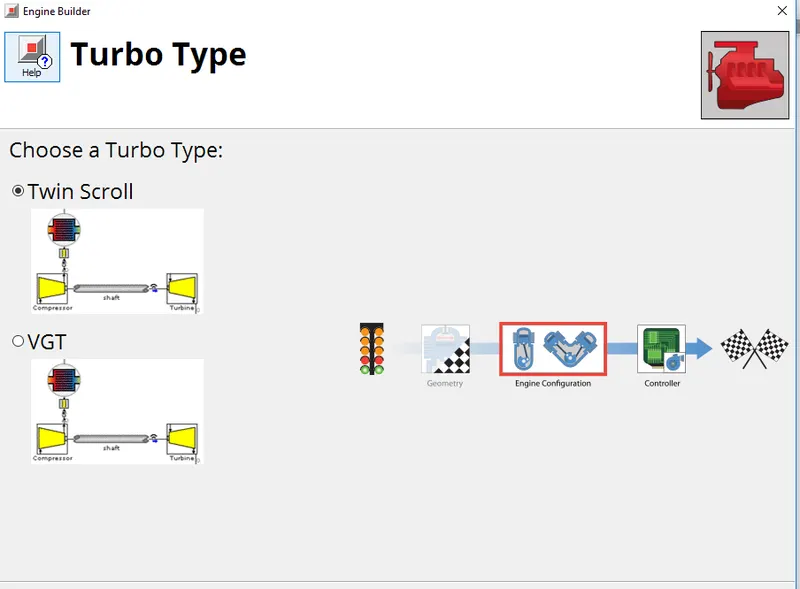
* When we click next we get a window where the type of turbo is set,

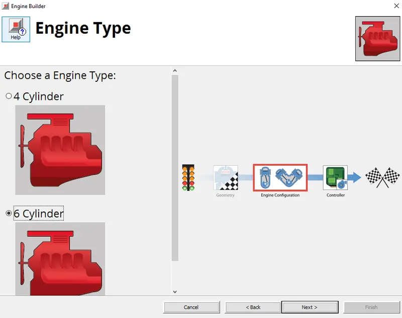
* By clicking next we define the number of cylinders,

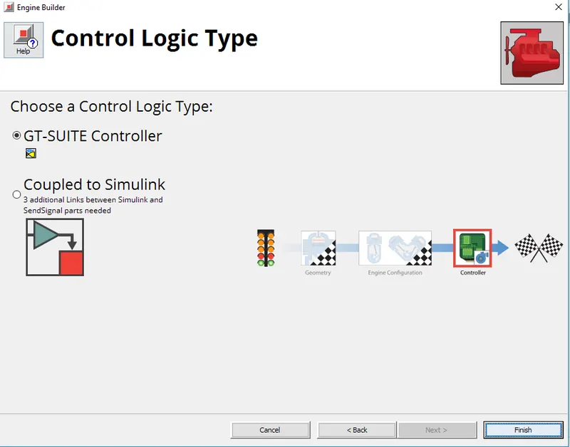
* In last window the controller type is set,

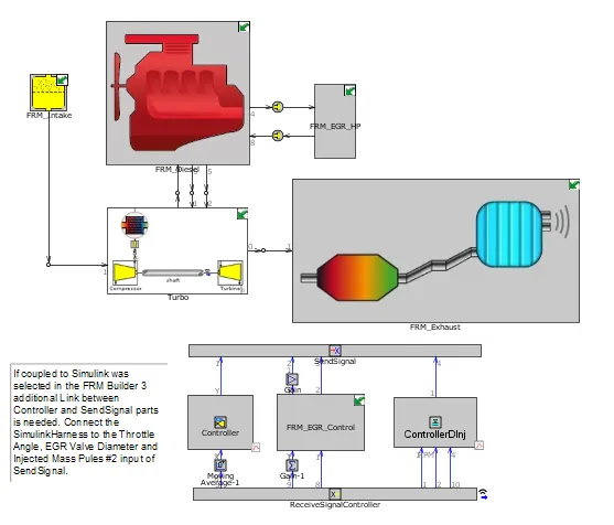
This gives us a engine model as shown below,

Result obtained as follows,

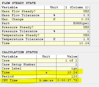
* If we compare the time taken to complete the simulation in the detailed model and also in the FRM, we see that the detailed model took less time and the FRM took more time, but the FRM took more time due to the number of periods for which the simulation is run. The FRM runs for 128 periods and the time required for this is 10.24 sec. But the detailed model ran for 75 periods and the time required for the same is 6 seconds, if the detailed model was run for 128 periods, the time required for this was more than 10 seconds.

* CPU time comparison even after running 128 periods of the FRM simulation took only 37.79 min, but the detailed model running for 75 periods took 1:53:56, which is almost 2 hours of CPU time.

* From the above result, it can be seen that FRM type simulations will be a good choice for Sil, Hil and Mil.