Week 1- Mixing Tee
Goal: To simulate T mixing for 2 different pipe lengths
Objective:
*Set up steady-state simulations
*Compare the mixing efficiency when the hot inlet temperature is 36 C and the cold inlet temperature is 19 C.
*Try both the k-epsilon and k-omega SST models for the first case and then use the best-fit model for further simulations.
*Simulate each case for a given velocity-to-momentum ratio
Case 1
*Short mixing T-shirt with a hot air supply speed of 3 m/s
*Momentum ratio 2.4.
Case 2
*Long mixing T-shirt with a hot air supply speed of 3 m/s.
*Momentum ratio 2.4
*Compare the results from the 2 cases on the number of cells, average outlet temperature and number of iterations for convergence.
*Plot the velocity and temperature contours on the section plane along and across the pipe.
*Also plot the velocity and temperature curves along and along the length of the pipe.
*Do an independent Mesh study for each individual case.
*In addition, discuss the effect of the length-to-momentum ratio on the results.
*Finally, show the convergence plot for each simulation
Introduction:
Mixing tees are widely used in the petrochemical industry in which two fluid streams with different physical and/or chemical properties are mixed. When there is a large temperature difference between the two streams, large fluctuations in metal temperature can occur in the area where the two streams meet unless proper design steps are taken. Temperature fluctuations in the metal can lead to thermal fatigue of the pipe at the pressure limit. If there is a crack through the wall, liquid may leak out, causing fire and damage. It is therefore necessary to ensure that the temperature fluctuations are such that the pipe system can withstand them. Options may include improving the mixing of the two streams to reduce temperature fluctuations by redesigning the piping system so that the momentum ratio of the two fluid streams is favorable for rapid mixing, or installing devices that protect the piping at the pressure limit.
A T-junction simulation is used here to evaluate the temperature change by mixing the same fluid at different temperatures and with different inlet velocities through two inlet pipes that are perpendicular to each other. The simulation is performed in two cases, only the geometry is different for each case (one is shorter than the other). We will also simulate a momentum ratio of 2 and 4 for each case.
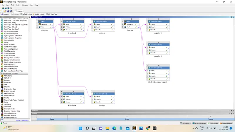
Gemoetry -> Mesh -> Setup -> Solution -> Results
Given data
Hot inlet temperature = 36 c
Cold inlet temperature = 19 c
Hot inlet velocity = 3 m/s
since, Mometnum ratio = Velocity of cold inlet / Velocity of hot inlet
Therefore,
For momentum ratio 2
Velocity of cold inlet = 6 m/s
For momentum ratio 4
Velocity of cold inlet = 12 m/s
Case 1 : SHORT MIXING TEE
Let's start by analyzing the best method for converging the solution for this particular case by studying two methods: k-epsilon and k-omega SST.
The above methods use simulation modeling of turbulence where the k-epsilon models predict the flow practically far from the boundaries (wall) and the k-omega model predicts near the wall.
The choice of model depends on the specific problem; no turbulent model suit just in case. Fine-tuning requires an SST model that used a fine mesh at the boundary and with the wall adjustment usually works in most cases; it is a specific problem.
Our first study sets up two settings, one for k-epsilon and one for k-omega SST. Here we use the same geometry and mesh for both simulation cases. So we use a short mixing tee model and mesh it.
Start the mesh setup by dragging to load the geometry and create the mesh.
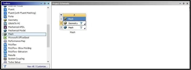
*Then open space claim to load geometry in setup. Space claim is a beneficial CAD cleanup software to prepare CAD geometry for simulation setup; it could be for FEA or CFD.
Therefore, load the geometry and extract the fluid volume (working fluid volume).
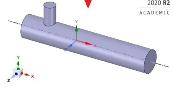
*Suppress the real model because we don't need to do any wiring simulation in this project. Finally, close the space claim.
Now we can get down to business. So click the mesh button to start Ansys meshing where we can generate the mesh and enter names for the entire surface of the geometry.
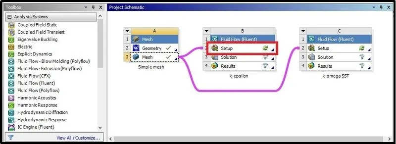
Next, create two smooth settings - one for k-epsilon and one for k-omega SST. Drag the output mesh into the Fluency Analysis Settings cell. Then update the mesh (right-click the mesh and use the update button) to convert and write the mesh for FLUENT analysis.
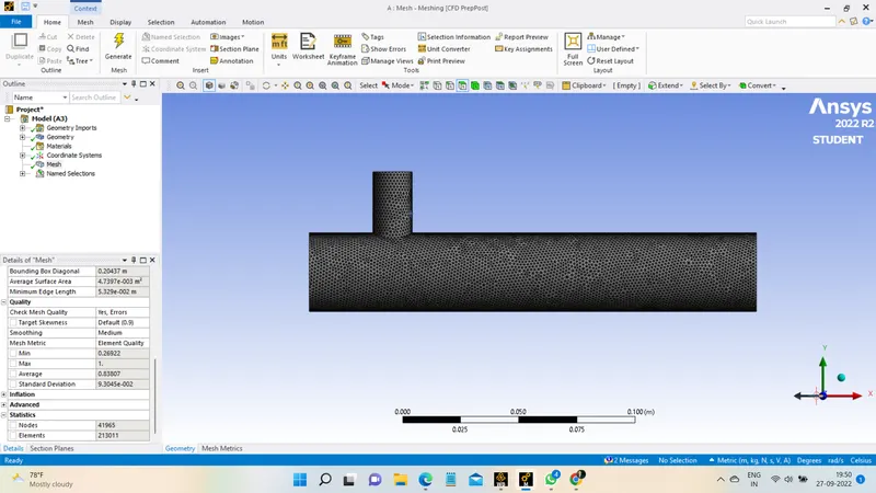
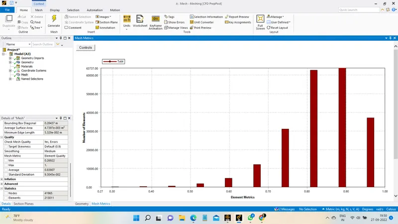
We can check our meshing by cutting the fluid domain into the section as shown below to observe mesh flow. And we can also investigate the quality of mesh by clicking on the option called element quality in the quality section of the mesh panel.
Then, double click on the setup option in the FLUENT cell for trying the k-epsilon method. It will open the FLUENT interface.
In Fluent, we will first see a console window that displays text and also accepts TUI (Text User Interface) commands. In the beginning we will see a lot of text about loading mesh cells, text about setting achromatic boundary conditions in the fluidity according to the name given to surfaces.
Once the domain geometry is fully loaded, it will display it in the GUI in a very striking way so that the user can understand what the imported boundary conditions will look like.
Next, in the domain panel, using the check button, we can check our network, which is suitable for smooth analysis or not. And we can improve the quality with the edit option.
After clicking the check mesh quality button, it will print the following conformation in the console window. Checking the mesh ensures that each cell is in the correct format and is connected to other cells as expected. It is recommended to check each network immediately after reading it. Failure of any check indicates a poorly constructed or corrupted network that will require repair before simulation.
Click on "units" to change the temperature units. FLUENT stores values in SI units. Most of the post-processing can be transferred to other units.
Then we set up the physics of the domain. Leave the general parameter settings as they are. Solver type -> pressure; speed formulation -> Absolute; solver time -> steady.
Next, activate the models. First, turn on the energy equation. Activating the energy equation makes it possible to solve the temperature-dependent problem.
In the viscus model, select 'k-epsilon', 'Realizable' for our first simulation type. Turbulence modeling is a complex field. The choice of model depends on the application. The Realizable k-epsilon model is used here, which is an improvement on the well-established standard k-epsilon model. Accept the remaining default settings.
In the cell zone, define the material, select the working fluid.
In "Boundary condition" click on "Inlet-x" and adjust the input parameter settings velocity to 3 m/s and temperature to 36oC. For input_y, set the velocity to 12m/s because we are using a momentum ratio of 2 and a temperature of 19oC.
Set the outlet pressure condition as the atmospheric pressure value, which is also zero gauge. The simulation may predict that the flow enters the model through a portion of the outlet. Backflow will bring turbulence and energy back into the model. However, the model cannot predict how much (because the flow comes from outside the model). It is therefore necessary to specify the return flow conditions. Ideally, the geometry should be chosen so that flow enters the model only at well-defined inlets. Backflow settings then do not affect the final solution (although they can be used in intermediate iterations).
In "Reports" press "new" to monitor surface reports. Select an area weighted average.
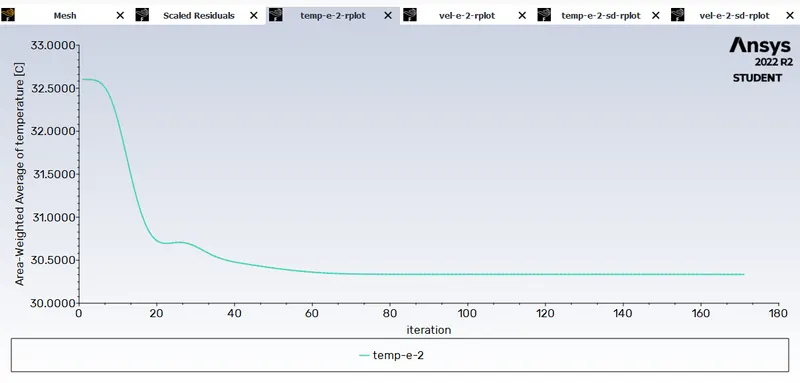
here we want the average temperature at the output surface, so select the temperature. And check "report file" and "report drawing".
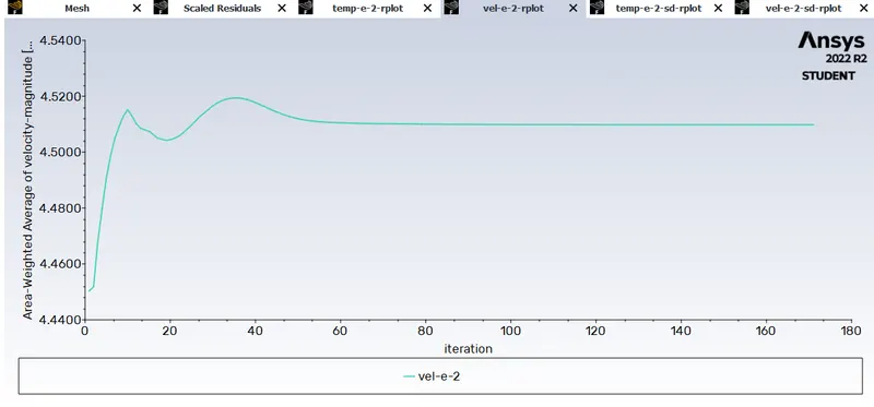
And in a similar way, create a plot of the average velocity in the output boundary conditions.
Before running the program, our last step will be to initialize the problem setup.
Initialization creates an initial solution that will be iteratively improved by the solver. In general, the same converged solution is achieved regardless of the initialization, although convergence is easier if they are similar. Basic initialization stores the same values in all cells. You can improve this in various ways - for example by patching different values into different zones. Some features, including patching and post-processing, are only available after initialization.
The hybrid initialization method is an effective solution initialization method based purely on simulation settings without the need for additional information. These methods produce a velocity field that corresponds to complex domain geometries, and a pressure field that corresponds to complex domain geometries, and a pressure field that smoothly blends high and low pressure values.
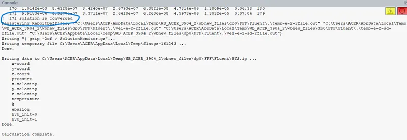
after pressing the initialize button the following will be printed in the console window saying that the initialization is complete.
Now we can run the simulation, just enter the number of iterations we want to run the simulation for and hit 'calculate'.
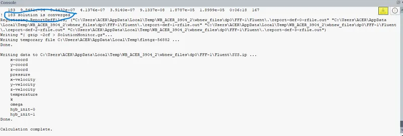
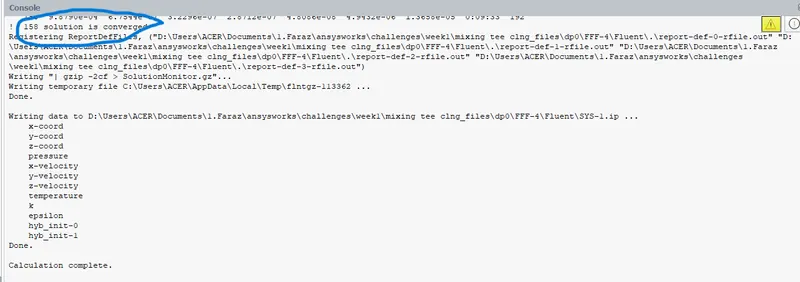
When the solution has fully converged, the following massage will be displayed Calculation completed.
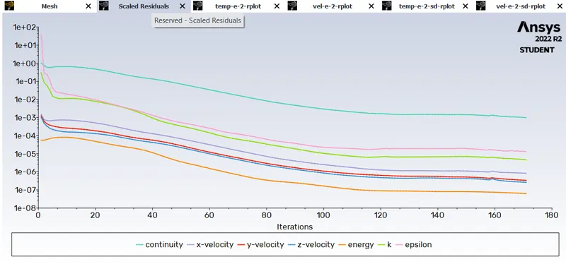
Calculating the solution also gives us our converged graph for the k-epsilon method. It also produced another output temperature and velocity report that we set earlier.
For moment ratio 2
(This is for k-epsilon SST model)
1.Convergence plot
2.Area-waited-average of temprature at outlet for each iteration
3.Area waited average of velocity-mag at outlet for each iteration
4.Standard deviation of temprature at outlet for each iteration
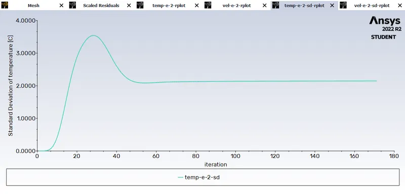
5.Standard deviation of velocity-mag at outlet for each iteration
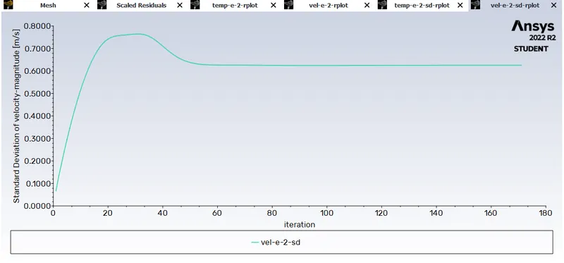
After that, we can close the flow and then process the results. Click on the results on the desktop and CFD-Post will open.
CFD-Post first displays the outline (wire model) of the model, which can be turned on by checking the surface displayed in the Outline panel of the fluid section.
The browser toolbar buttons allow you to manipulate the view.
Create a plane - from the location menu select 'Plane' -> accept default name 'Plane 1' -> set 'Method' to 'YZ Plane', accept 'X' as 0.0 and press 'Apply'
6.For temprature contour.
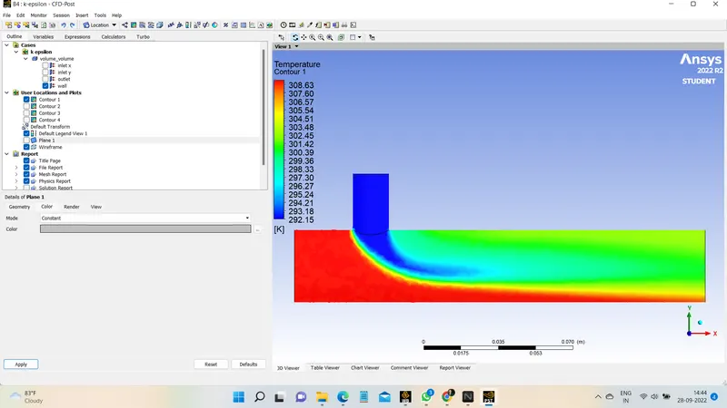
7.Now, for velocity contour.
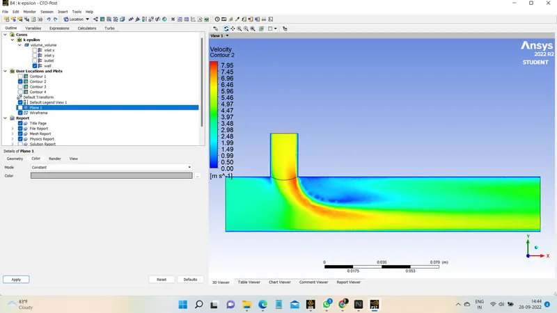
8.Number of Iteration taken for covergence is
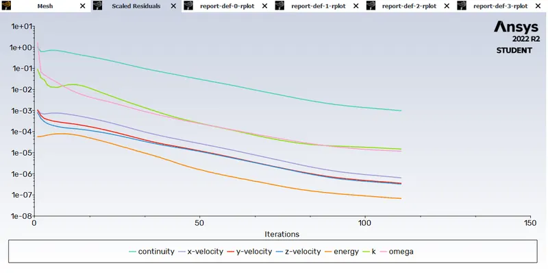
This time, we are going to use the same setting for the next simulation and solve the problem by the k-omega SST method. And compare all the results
1.Convergence plot
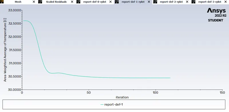
2.Area waited average of temprature at outlet for each iteration
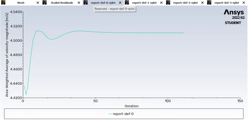
3.Area waited average of velocity-mag at outlet for each iteration
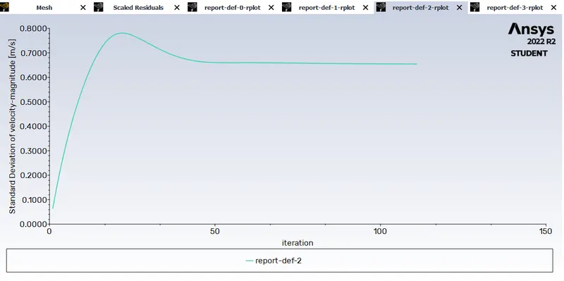
4.Standard deviation of temprature at outlet for each iteration
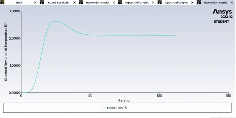
5.Standard deviation of velocity-mag at outlet for each iteration
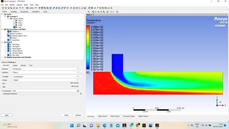
6.For temprature contour.
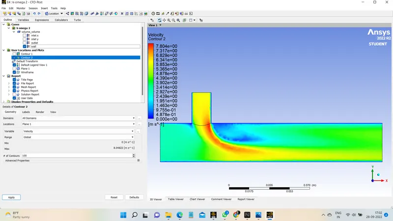
7.Now, for velocity contour.
8.Number of Iteration taken for covergence is
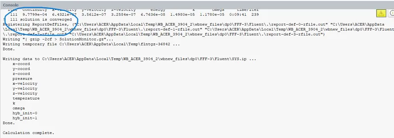
For moment ratio 4
For k-epsilon SST model
1.Convergence plot
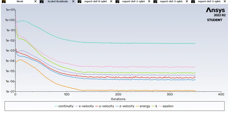
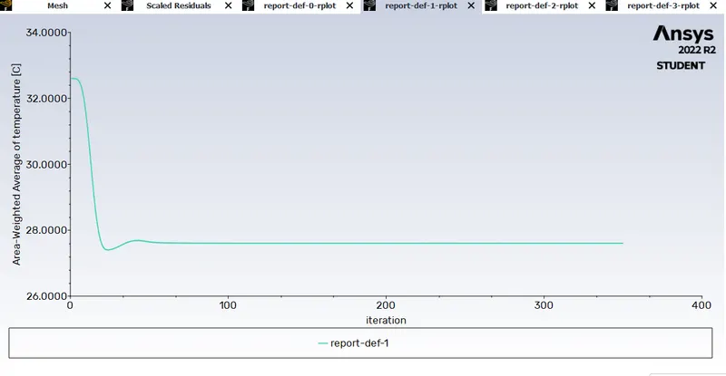
2.Area waited average of temprature at outlet for each iteration
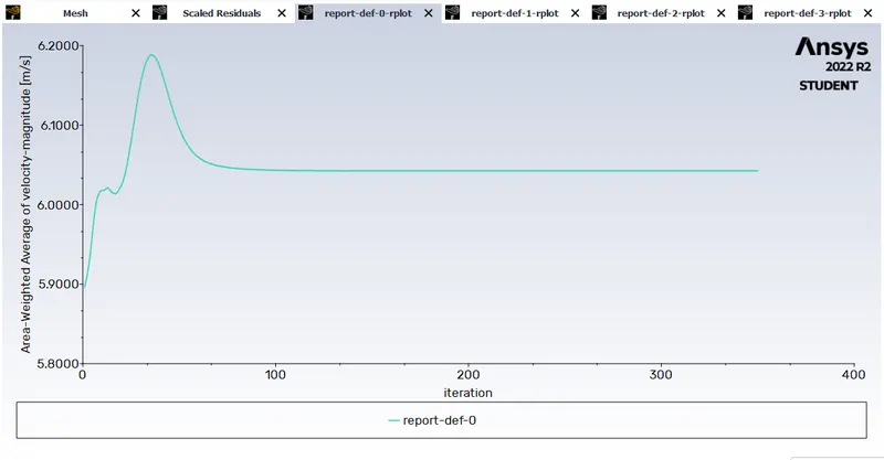
3.Area waited average of velocity-mag at outlet for each iteration
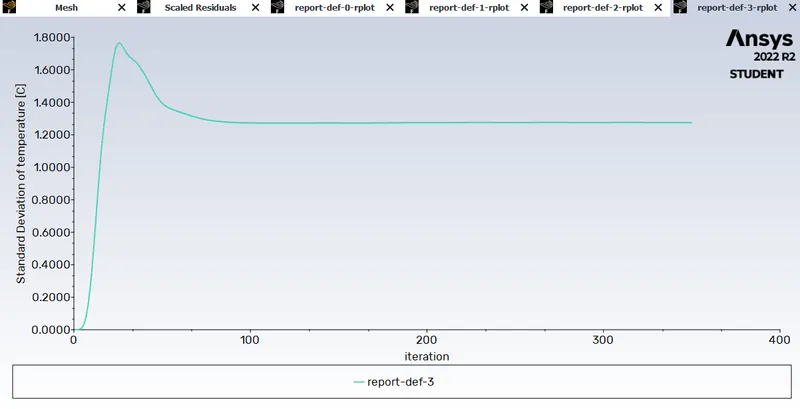
4.Standard deviation of temprature at outlet for each iteration
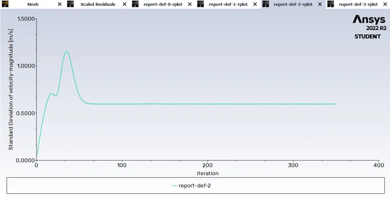
5.Standard deviation of velocity-mag at outlet for each iteration
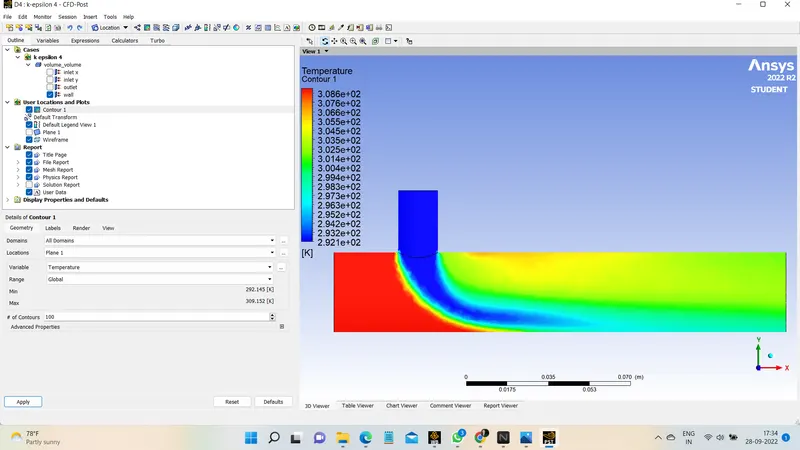
6.For temprature contour.
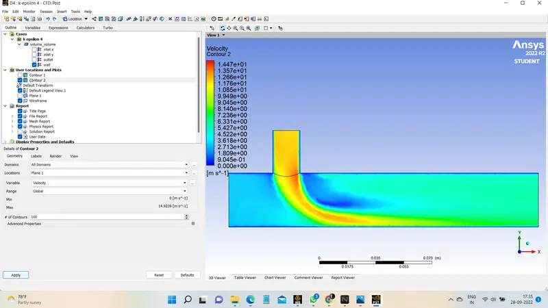
7.Now, for velocity contour.
8.Number of Iteration taken for covergence is
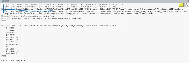
For k-omega SST model
1.Convergence plot
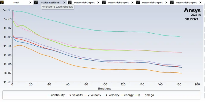
2.Area waited average of temprature at outlet for each iteration
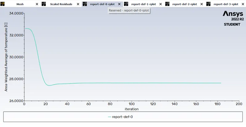
3.Area waited average of velocity-mag at outlet for each iteration
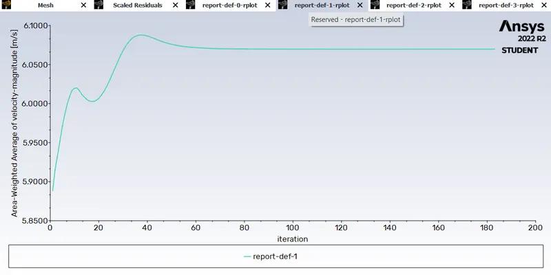
4.Standard deviation of temprature at outlet for each iteration
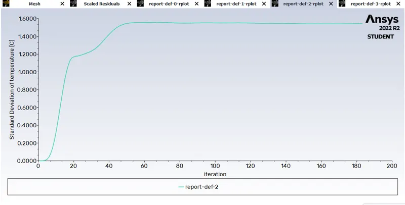
5.Standard deviation of velocity-mag at outlet for each iteration
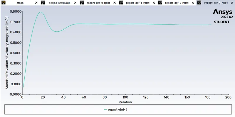
6.For temprature contour.
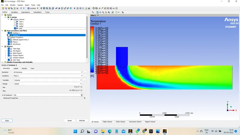
7.Now, for velocity contour.
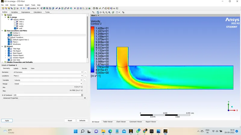
8.Number of Iteration taken for covergence is
For further calculation
The k-omega model is suitable for simulating flow in a viscous sublayer. Conversely, the k-epsilon model is ideal for predicting flow in regions away from the wall
The SST model shows less sensitivity to free-stream conditions (flow outside the boundary layer) than many other turbulence models.
The shear stress limiter helps the k-omega model avoid the accumulation of excessive turbulent kinetic energy near stagnation points.
If we observe our simulated figure, we can notice that in the k-omega model the flow is rather laminar and does not give the correct turbulent results, whereas the k-epsilon simulation gives the correct mixing of both air streams.
In this particular case, we are not dealing with walls, so we will use the k-epsilon method for further simulations.
Case 2 : LONG MIXING TEE
For moment ratio 2
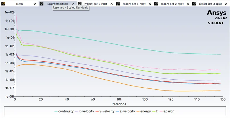
1.Convergence plot
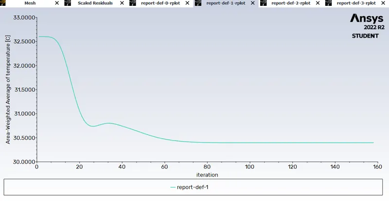
2.Area waited average of temprature at outlet for each iteration
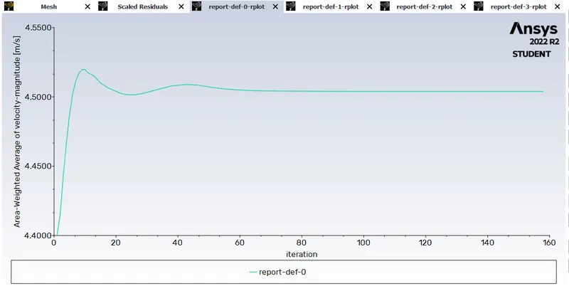
3.Area waited average of velocity-mag at outlet for each iteration
4.Standard deviation of temprature at outlet for each iteration
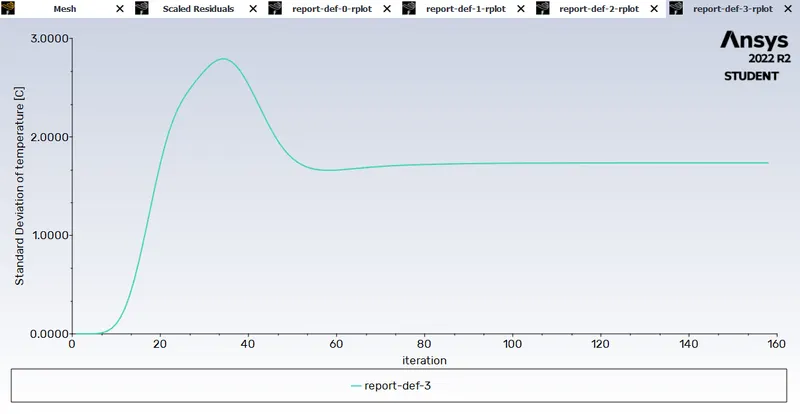
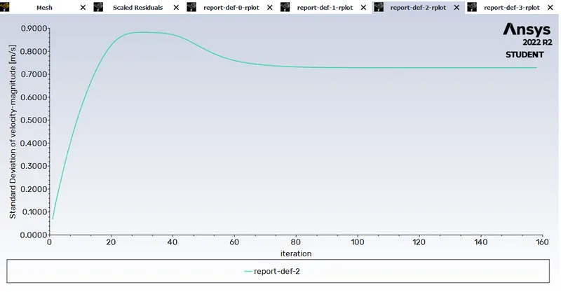
5.Standard deviation of velocity-mag at outlet for each iteration
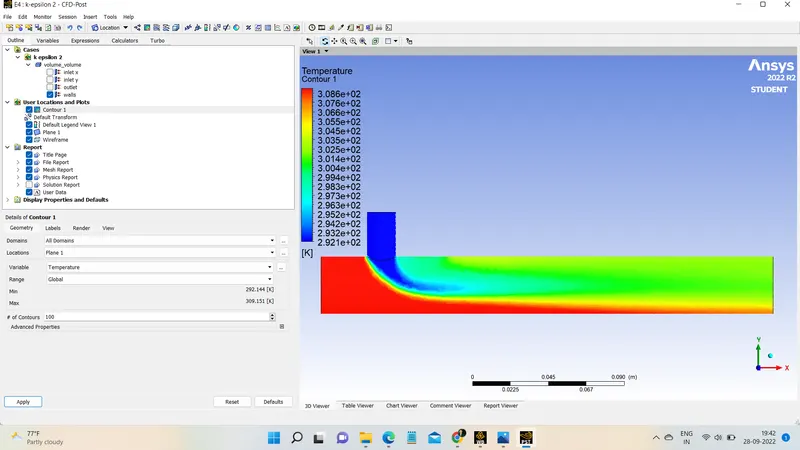
6.For temprature contour.
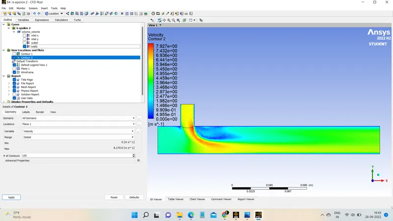
7.Now, for velocity contour.
8.Number of Iteration taken for covergence is
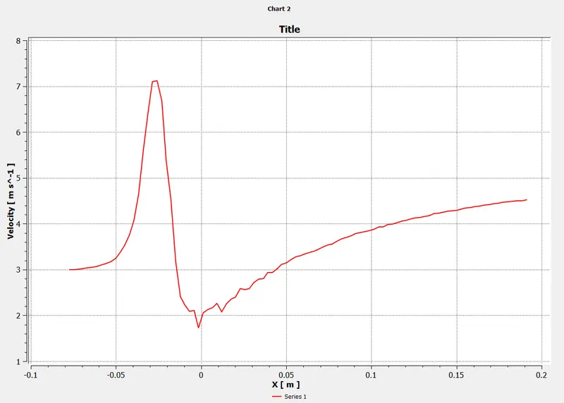
9.Velocity line plot along the length of the pipe.
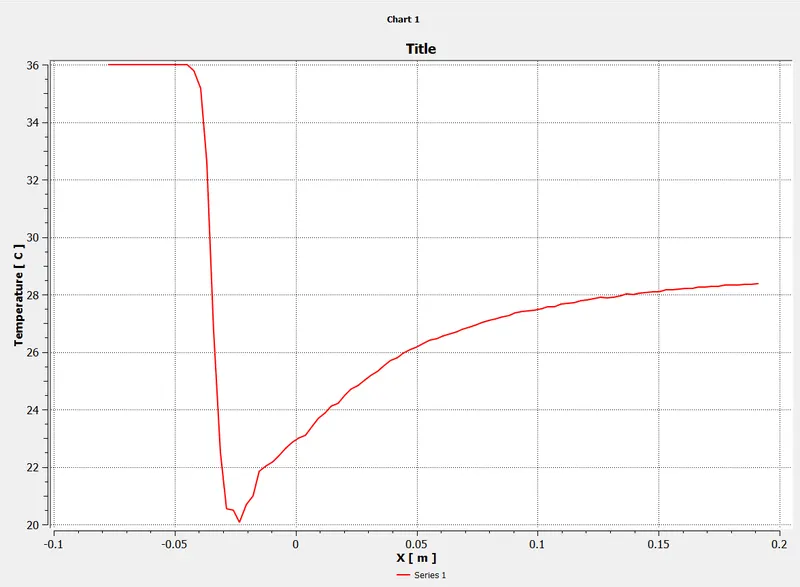
10.Temperature line plot along the length of the pipe.
For moment ratio 4
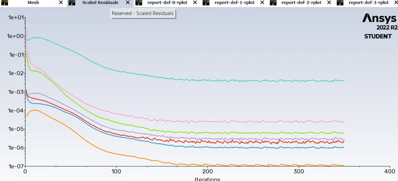
1.Convergence plot
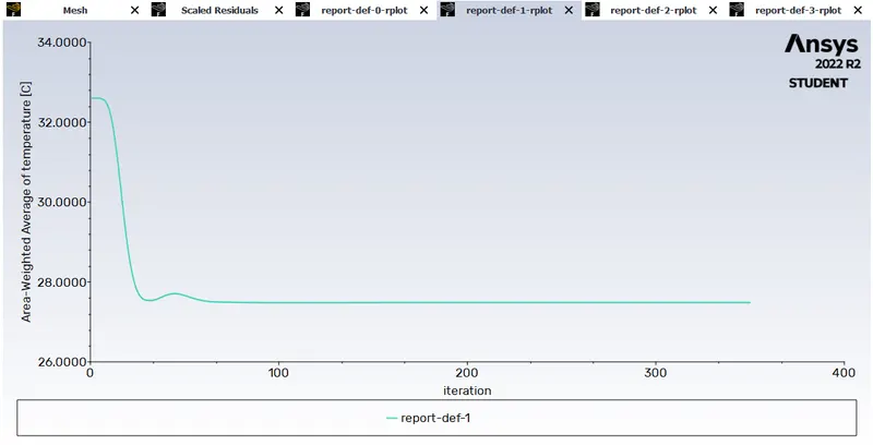
2.Area waited average of temprature at outlet for each iteration
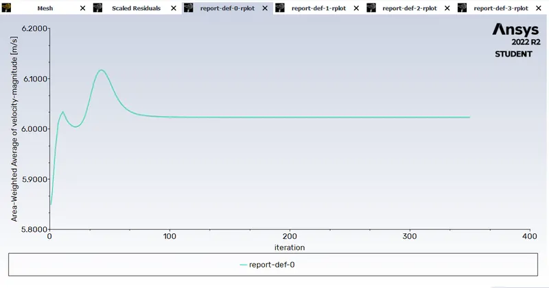
3.Area waited average of velocity-mag at outlet for each iteration
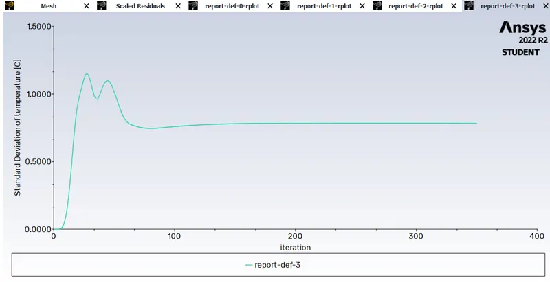
4.Standard deviation of temprature at outlet for each iteration
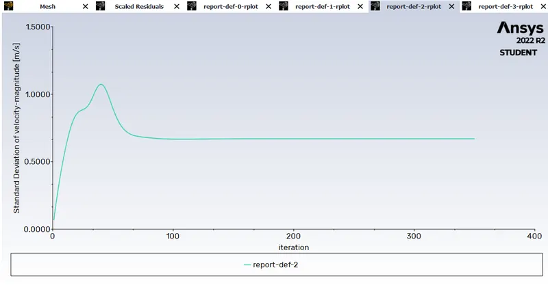
5.Standard deviation of velocity-mag at outlet for each iteration
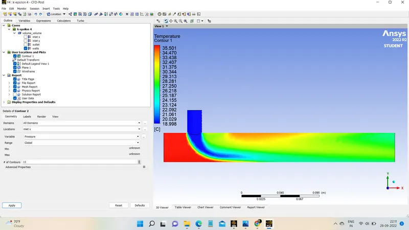
6.For temprature contour.
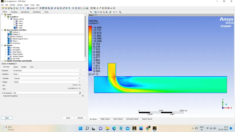
7.Now, for velocity contour.
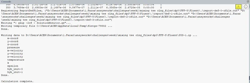
8.Number of Iteration taken for covergence is
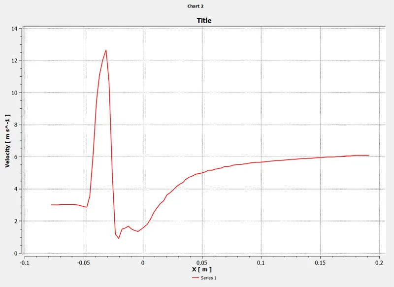
9.Velocity line plot along the length of the pipe.
10.Temperature line plot along the length of the pipe.
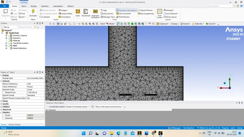
Mesh independent study for long tee of momentum ratio 4
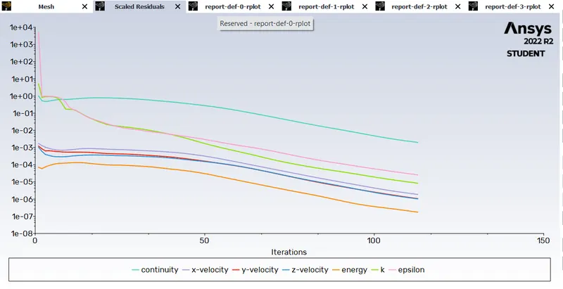
1.Convergence plot
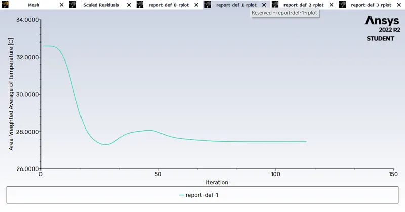
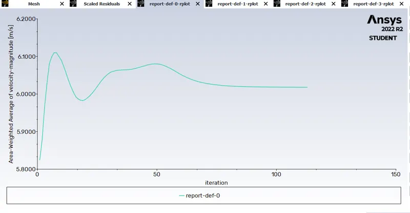
2.Area waited average of temprature at outlet for each iteration
3.Area waited average of velocity-mag at outlet for each iteration
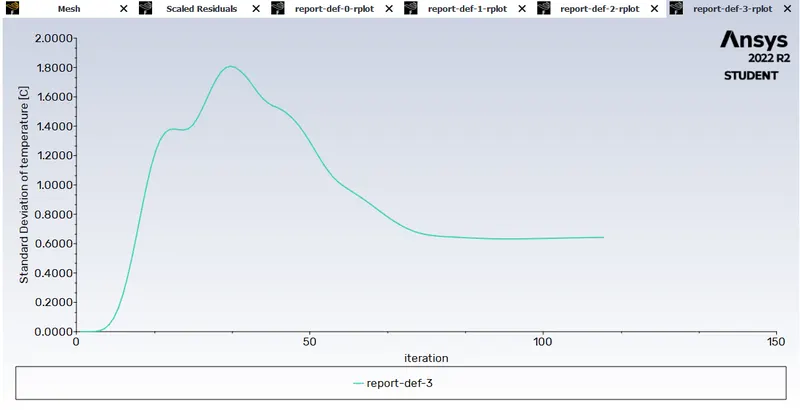
4.Standard deviation of temprature at outlet for each iteration
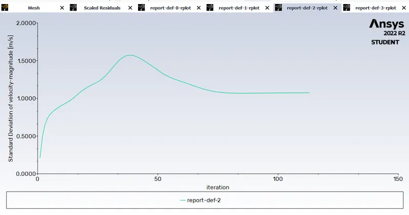
5.Standard deviation of velocity-mag at outlet for each iteration
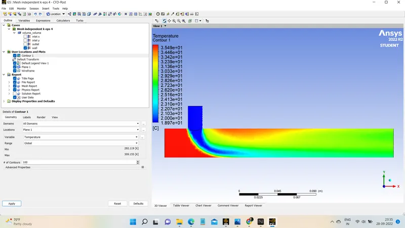
6.For temprature contour.
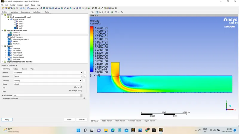
7.Now, for velocity contour.
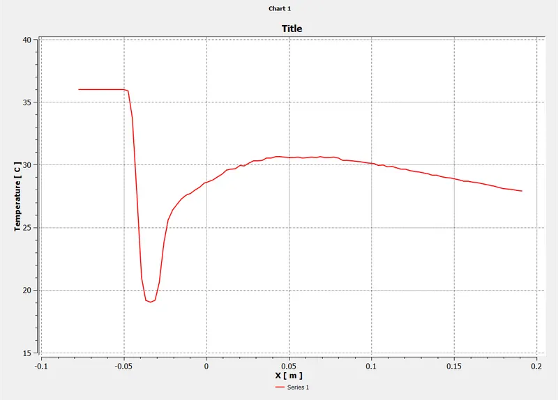
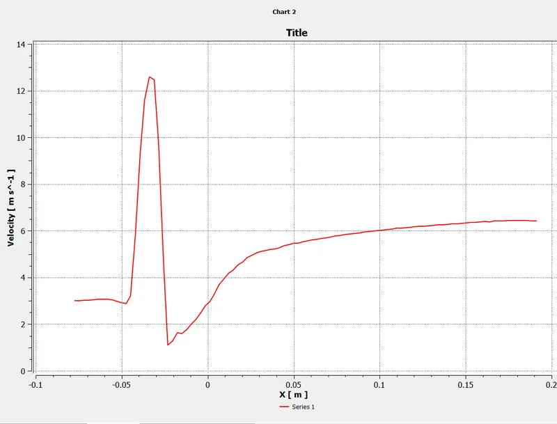
8.Velocity line plot along the length of the pipe.
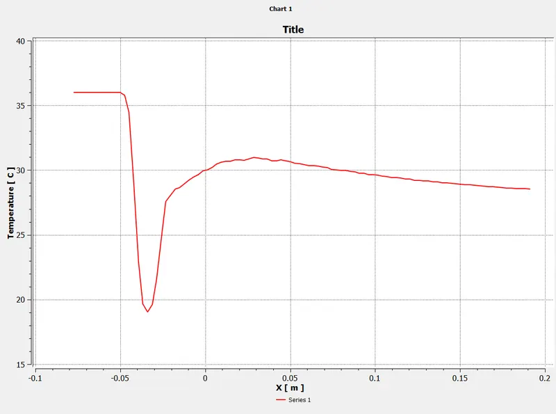
9.Temperature line plot along the length of the pipe.
Workflow
Effect of length and Momentum ratio
| Momentum ratio | Pipe length | Outlet temperature |
| 2 | Short | 302.159 k |
| 4 | Short | 301.737 k |
| 2 | Long | 302.654 k |
| 4 | Long | 302.039 k |
| 4 | Long(inflamation) | 302.221 k |
Conclusion:
*It can be observed that when the momentum ratio is 4, i.e. when the cold inlet velocity is 12 m/s, there can be a slight drop in temperature compared to the momentum ratio of 2.
*This is true for both cases. This is due to the fact that as the cold inlet velocity increases, there is more turbulent mixing, which further lowers the temperatureSo comparing the temperature standard deviation of the short and long pipes with a momentum ratio of 4.
*it was observed that there was a smaller deviation for the long pipe (graphs are where appropriate). Therefore, it is recommended to use a long pipe for efficient mixing