Week 5 - Rayleigh Taylor Instability

Goal: Study and simulation of Rayleigh Taylor instability using the VOF method.

Objective:

• Explore the significance of the Rayleigh Taylor instability
• ANSYS FLUENT multiphase flow analysis.
• Explore the approach to fluid volume and its importance.
• Investigating how mesh refinement affects the Rayleigh Taylor instability
• Investigate and calculate the Atwood number for density difference modeling.
• Describe the instability behavior based on Atwood numbers.

Introduction:

When applied to the flow of pipelines and other transport media, single-phase fluid flows predominate. Multiphase flows have recently been introduced into industrial development applications and are growing in popularity. Multiphase flow refers to the idea of ​​performing a task using two or more different fluids, whether or not they are miscible. Depending on the application, a multiphase flow can consist of two liquids that are identical but have different densities, or it can be a gas-liquid flow. Multiphase flows are used in the chemical industry, nuclear industry, manufacturing facilities and product mixing.

The Rayleigh Taylor instability is one sector of multiphase flow that is based on density stratification in which a heavier fluid is on top of a lighter fluid that is inherently unstable. A small perturbation can be induced at the interface to allow the fluid to move in the gravitational field. The cause of instability is mostly dependent on the density of both liquids. The governing equation, which resembles the Rayleigh Taylor instability in 2 dimensions, is mostly assumed based on two immiscible liquids, i.e., the viscosity of the liquids is not considered. In such an unstable state, the fluid is always trying to reach an equilibrium position and therefore can be monitored with respect to time. The Rayleigh Taylor instability equation is both linear and nonlinear in nature. Linear in nature when the perturbations or perturbations are small and non-linear in nature when the perturbations are high. Rayleigh Taylor instability is common in real life, one of the best examples being oil floating on water. From which we know that oil with higher density and water with lower, oil always floats above water from now on. Another application of the Rayleigh Taylor instability can be seen in plasma fusion reactors and fusion in confined space where inertial effects dominate. In space, we can also see the Rayleigh Taylor instability in a supernova explosion as well, where a single star can collapse when the mass in the core increases significantly, where the gravitational force increases and causes collapse due to differences in mass and densities. Mushroom clouds are another example of the Rayleigh Taylor instability, in which there is a sudden formation of large, low-density gases at any particular height.

The Rayleigh Taylor instability has been used for many other CFD codes to run the simulation. Because we know that depending on the density of the liquid, the change in the flow of the liquid can be different also depending on the flow rate and turbulence, the generation of plateaus can be different, and therefore different models are developed. Those models are:

Saffman-Taylor instability
Viscosity pinching, a morphologically unbalanced interface between two fluids that occurred in porous media, is another name for this instability. This phenomenon is primarily seen through the drainage processes of soil media. The more viscous fluid is further displaced downward to create a fingering effect when the less viscous fluid is injected. This instability is also caused when no forced displacement is offered, therefore it also affects the gravitational force as RT instability.

Richtmyer-Meshkov instability
The Richtmyer–Meshkov instability, unlike the Rayleigh Taylor instability, is caused by an external force and is driven by the acceleration of the fluid. When two fluids of different viscosity and density are impulsively accelerated, this instability develops. This instability begins as a small perturbation, increases linearly over time, and then enters a nonlinear phase, during which bubbles appear in the lighter liquid as it penetrates the heavier liquid and spikes form in the higher density liquid as it penetrates the lower density liquid. After a turbulent period, the two fluids combine. Examples of the Richtmyer–Meshkov instability include inertial confinement fusion, where the instability is caused by the acceleration of hot mantle material towards the fuel layer. Another example of Richtmyer-Meshkov instability in scramjet engines

Plateau-Rayleigh instability
Plateau-Rayleigh In more specific aspects, the instability is more like the Rayleigh Taylor instability. The mixing of two liquids can vary depending on the type of liquid used and the interference used. The main focus of this instability is the breakup of the fluid filament, part of fluid dynamics. The process of breaking a liquid bubble into several pieces due to surface tension and contact area is known as liquid fiber breakup. a simulation that focuses more on the Plateau-Rayleigh instability is the motion of an ink jet through air or another liquid. This simulation allows us to observe the bursting of an ink bubble as it passes through a fluid of reduced density. Water leaking from faucets and inkjet printers are two common examples of this instability.

• The Atwood number (A)It is a dimensionless number in fluid dynamics used in the study of hydrodynamic instabilities in density stratified flows. It is a dimensionless density ratio defined as

  

  where

   = density of heavier fluid

   = density of lighter fluid

Modeling approach:

The simulation approach is very simple and is a 2D analysis in which two surfaces are attached to each with an interface between them. The solution methodology is created based on the goal defined for the simulation. The simulation will take place in 4 different cases which are:

Case 1: - Mesh size 0.5 mm for water and air as starting material.
Case 2: - Mesh size 0.1 mm for water and air as starting material.
Case 3: - 0.1mm mesh size for water as default material and one user defined material.
   As long as two fluids are present, a multiphase simulation will be performed. For the multiphase procedure, we will use the Volume of Fluid approach, which is well known for sloshing simulations. We have previously discussed the existence of a phase interface between two liquids that may or may not be immiscible. It is essential to develop a mechanism that accurately predicts the kinematic motion of the fluid interface in order to monitor it. Moving grid method, marker particle methods, and VOF method are commonly used methods in FLUENT to track interfaces. Small free surface deformation is typically treated using a moving grid or an adaptive grid. Large deformation problems cannot be handled by this method, which requires a change in network topology. Using polynomials and nearby marker particles, the interface is tracked in the case of the marker technique. However, it can only be used for short 2D simulations. The Volume of Fluid technique offers a 3D interface with excellent volume preservation. In the VOF model, we cannot have two fluids with the same density because they will interact at the molecular level. The interface of the VOF model cannot be smaller than the volume mesh, which is its only limitation.

Geometry :

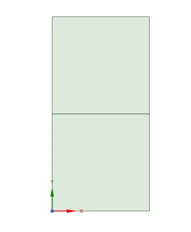
• Geometry is created in spaceclaim with a dimension of 20x20.
• Two squares has been created in such a way that it is placed one over the other.
• After that pull tool is used to convert a sketch into surfaces.
• Then share the topology between two surfaces for the effective transfer of information and to connect  a mesh between two interfaces.

Mesh :

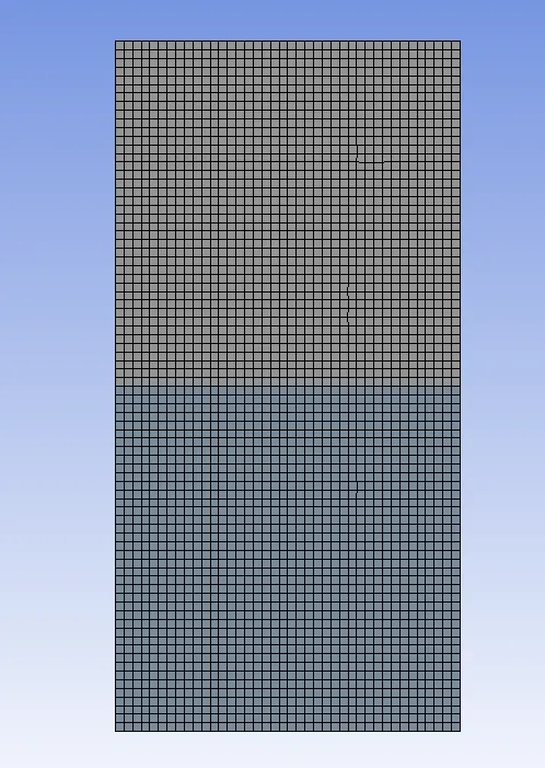
Case 1 :

Details :

Mesh	Coarse
Element size	0.5 mm
Number of elements	3200
Density of primary fluid	Air (1.225 kg/m3">m3m3)
Density of secondary fluid	Water (998.2 kg/m3">m3m3)
Atwood number	0.9975

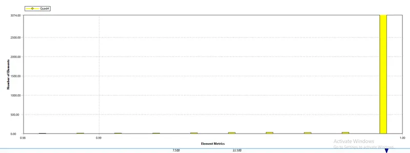
Mesh quality :

 

STEP 3 : SETUP

SETUP
Solver Type	Pressure-Based
Velocity Formulation	Absolute
Time	Unsteady
Models	Viscous model : laminar Multiphase      : Volume of fluid                      : Implicit formulation                      : 2 phases
Material	Fluid type   : Air                   : water liquid  Solid-type   : Aluminium
Cell zones	Fluid type  : Air                  : water
Boundaries	Standard
Reference values	Standard
Initialization	hybrid
Patch	Water-surface (1 value of volume fraction of water)  Air-surface (0 value of volume fraction of water)

 Residual plot :

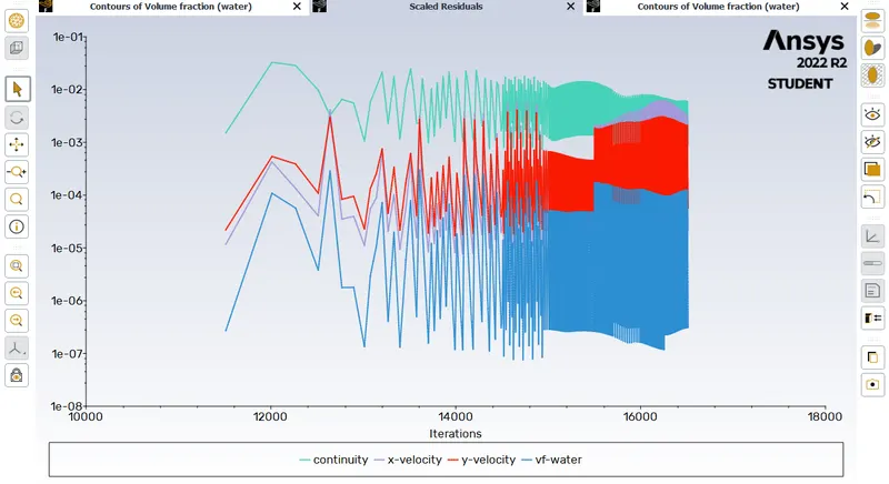
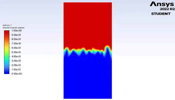
youtube link for case 1:https://youtu.be/lgjMMZU2n2s

GIF:

Case 2 :

Details :

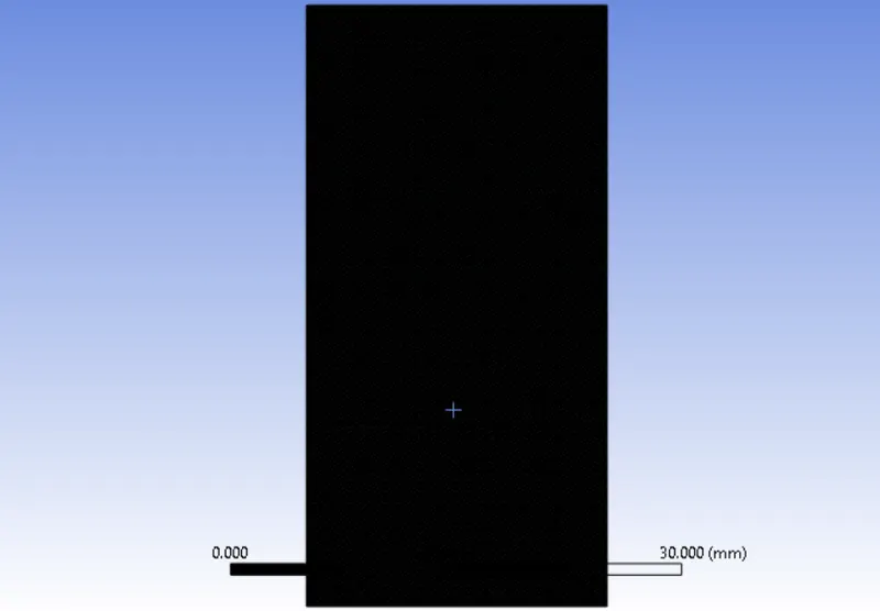
Mesh	Refined
Element size	0.1 mm
Number of elements	80000
Density of primary fluid	Air (1.225 kg/m3">m3m3)
Density of secondary fluid	Water (998.2 kg/m3">m3m3)
Atwood number	0.9975

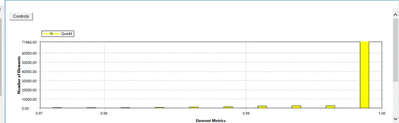
Mesh quality :

STEP 3 : SETUP

SETUP
Solver Type	Pressure-Based
Velocity Formulation	Absolute
Time	Unsteady
Models	Viscous model : laminar Multiphase      : Volume of fluid                      : Implicit formulation                      : 2 phases
Material	Fluid type   : Air                   : water liquid  Solid-type   : Aluminium
Cell zones	Fluid type  : Air                  : water
Boundaries	Standard
Reference values	Standard
Initialization	hybrid
Patch	Water-surface (1 value of volume fraction of water)  Air-surface (0 value of volume fraction of water)

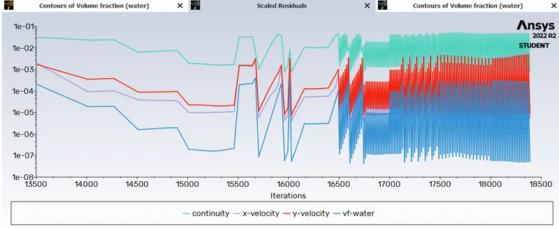
Residuals :

Youtube link for case2:https://youtu.be/dq5Weqi2n1g

GIF:

Case 3 :

Details :

Mesh	Refined
Element size	0.1 mm
Number of elements	80000
Density of primary fluid	User-defined material (400 kg/m3">m3m3)
Density of secondary fluid	Water (998.2 kg/m3">m3m3)
Atwood number	0.4278

Mesh:

Mesh quality:

STEP 3 :

SETUP
Solver Type	Pressure-Based
Velocity Formulation	Absolute
Time	Un-Steady
Models	Viscous model : laminar Multiphase      : Volume of fluid                      : Implicit formulation                      : 2 phases
Material	Fluid type      : user-defined                      : water liquid  Solid-type      : Aluminium
Cell zones	Fluid type      : Air                      : water
Boundaries	Standard
Reference values	Standard
Initialization	hybrid
Patch	Water-surface (1 value of volume fraction of water)  Air-surface (0 value of volume fraction of water)

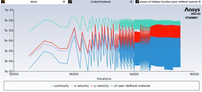
Residual :

Youtube link for case 3:https://youtu.be/bCTwoZb4hiw

GIF:

conclusion:

Why not a steady state solution:
Although a steady-state simulation can also be solved, the VOF model is typically used to solve time-dependent problems. Only when our solution is independent of the initial conditions and specific inflow and outflow boundary conditions for each phase are present can a steady-state simulation of the VOF model make sense. The steady-state solution is used only when results are needed at the end of a time step and no intermediate results are needed. It is important to ensure that the volume fraction is a function of time in the case of instability, as it will vary with time.

The effect of the mesh on the results
The area-weighted average water volume fraction decreases earlier in the basic network configuration, and as the network size decreases, the decrease progresses in time. This suggests that as the number of elements increases, we better capture the flow phenomena. We can therefore conclude that the mesh size affects how the hydrodynamic instability converges. In addition, it was found that the number of simulation iterations increased by a factor of 2.5 to 3 as the mesh size decreased.

Atwood number comparison
In cases 1 and 2, Atwood's number approaches 1, while in the case of user-defined content it was almost halved. The stratification effect is more pronounced when the Atwood number approaches 1, which means that the mixing is essentially symmetric. As we increase the material density in the case of the user-defined material, the mixing effects decrease and only a small plateau is visible in the simulation.

Comparison of animation
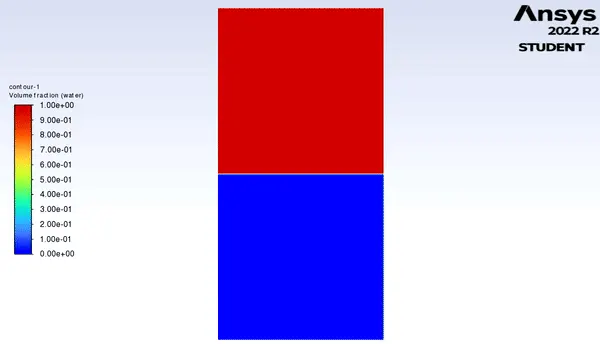
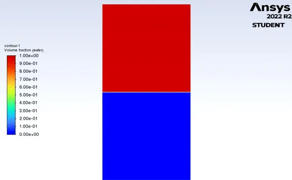
Case 1 showed very clearly that the lack of network elements causes very rapid mixing and a rapid gain in equilibrium for both liquids. In the latter case, we can observe that the mixing is slower and that more iterations are needed to complete the simulation. In the third scenario, the mixing is very slow and we can see more clearly how the water moves down due to gravity. User-defined content was introduced in the fourth example. In this case, water interacting with a user-defined material results in the creation of a mushroom shape.