Week 2 - Flow over a Cylinder.
TARGET:
Simulate the flow over a cylinder and explain the Karman vortex street phenomenon. Understanding the vortex for different Reynolds numbers corresponding to varying inlet velocities. Create a monitoring point behind the cylinder at a distance of four times the diameter that can be used to calculate and analyze vortex shedding.
OBJECTIVE:
1. Simulate flow with steady and unsteady case and calculate Strouhal number for Re= 100
2. Calculate the drag and lift coefficient over the cylinder by setting Reynolds number to 10,100,1000,10000 & 100000. (Run with steady solver)
2. Discuss the effect of Reynolds number on drag coefficient. [The results should be validated using any standard literature and the error should be within 5%]
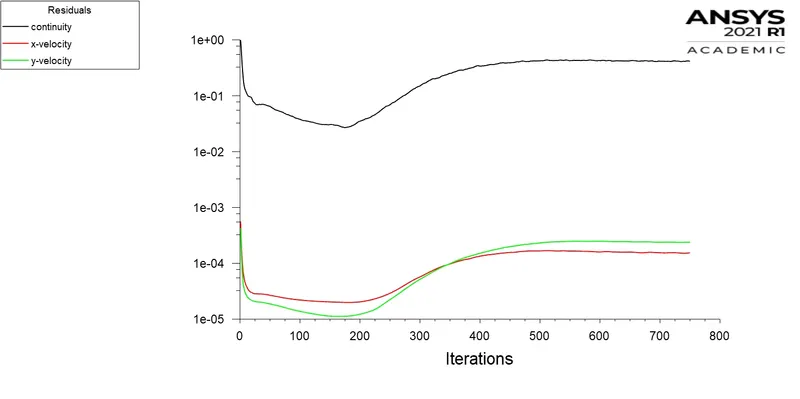
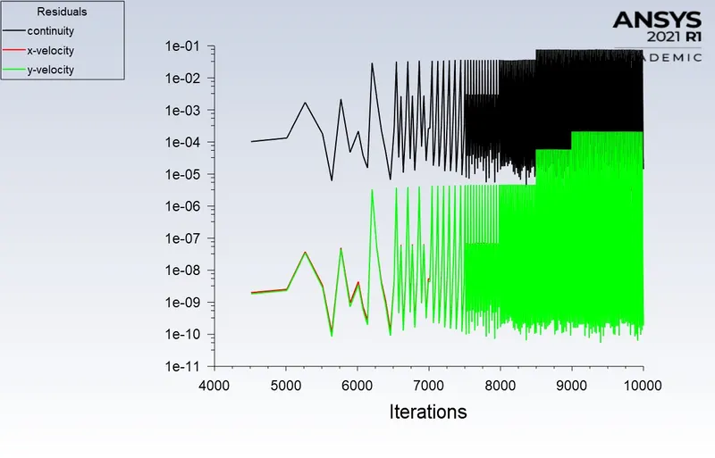
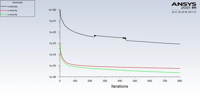
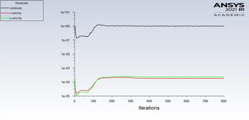
3. In both approaches, show that the flow has converged. That is, what quantities or graphs do we need to look at to determine that the flow has converged?
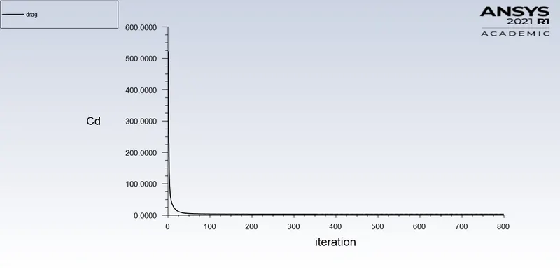
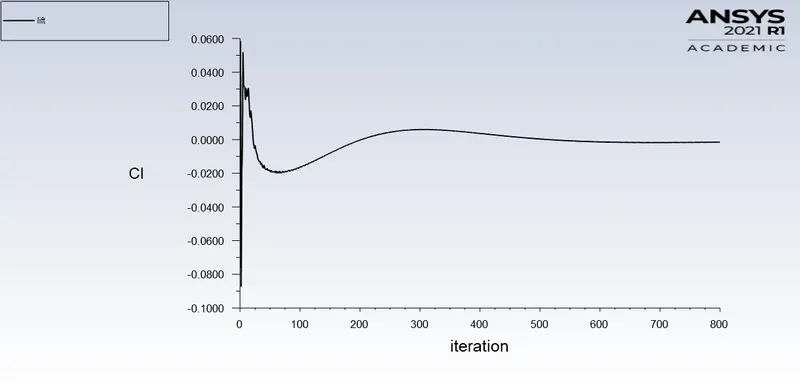
4. Graphs of drag and lift coefficient.
5. Graphs showing vortex shedding behind the cylinder.
6. At the bottom of the prompt page, indicate your preferred material.
introduction:-
Flow over a cylinder is one of the fundamental simulations in the CFD domain, and to this day research continues to study the unsteady behavior caused by the flow. The study of flow over a cylinder is very complex and a periodic flow pattern is seen at lower Reynolds number and after reaching a critical value of Reynolds number the flow changes into a wake region and this wake formation can be studied using Von karman vortex street literature. If we consider any other object compared to a cylinder, most of them will cause boundary layer separation due to the effect of geometrical properties such as sharp edges, but in the case of a cylinder this separation point is very complex and depends on the nature of the upper boundary layer and other parameters flow.
The laminar region to the turbulent region is governed by a dimensionless number called the Reynolds number, which is the ratio of inertial forces to viscous forces. This number is a measure of various flow criteria in an area that can be calculated from the fluid flow density, flow velocity, characteristic linear dimension depends on the geometry and dynamic viscosity of the fluid. Since the flow in the wake region can have a periodic motion, it can have a certain frequency at which it resonates. If this frequency coincides with the structural frequency of the object, it can cause a phenomenon called resonance. This frequency of motion can be given by another dimensionless number called the grater number, which is used to determine the frequency over the flow. The relationship between the Reynolds number and the grater number can be used to determine the time step for the simulation, since for a particular Reynolds number the grater number is given in many literatures.
Vortex-induced vibrations are one of the key aspects that can lead to the study of vortex shedding in real-world applications such as bridges, aircraft control surfaces, heat exchangers, and many others. Vibrations caused by vortex phenomenon due to flow dynamics need to be studied for very good scale product design and development. The Strouhal number is also used with another number in an axial flow turbine to determine the blade frequency during the flow period.
Solution and Modeling Approach:-
The main goal of the project is to study the behavior of the Reynolds number on the flow through a cylinder. To capture the flow with each mode, it is important to have a larger flow domain and a smaller mesh size to capture every possible vortex in the wake region.
The problem is divided into two groups, in which steady state and unstable state simulation will take place. In a steady state simulation, the variable Reynolds number will be accounted for by keeping the fluid property constant. The simulation will run for 10,100,1000,10000 and 100000 Reynolds numbers and other parameters will be studied accordingly. The problem will start with the 2D flow field and mesh geometry. It is important to have a smaller mesh size to capture all the small details from the flow domain. An inflatable layer will be added near the cylinder to capture the separation of the boundary layer from the cylinder surface. Since this is a steady state simulation, this project will include a special method to solve the problem with the traditional and NITA method, i.e. non-iterative time shift. This solver is more focused on solving the time march problem with greater ease and with fewer iterations. The boundary conditions will be as simple as velocity inlet and pressure outlet with wall type symmetry. A cylinder will also be considered as a wall type on which the lift and drag coefficients will be calculated.
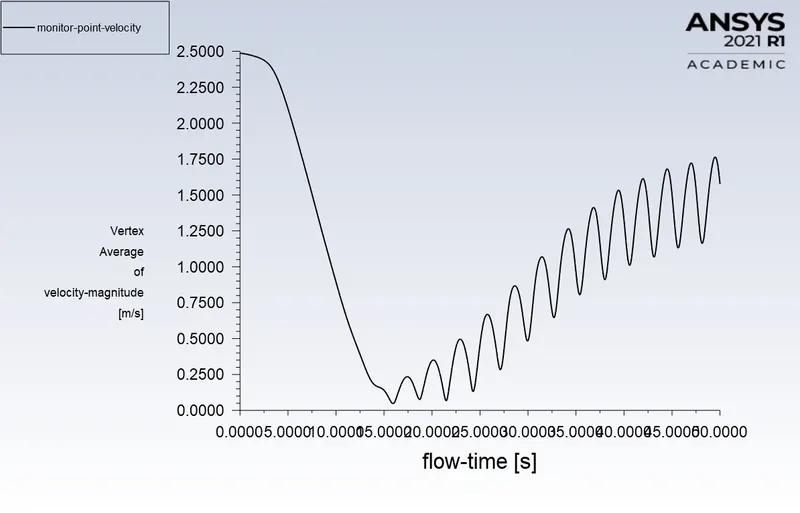
For the steady solver, a simple interpolation scheme will be used to calculate the results in the adjacent volume. The simulation of the non-stationary state will be performed using two interpolation schemes, one is SIMPLE and the other is PISO with NITA. To check the convergence of the solution, we create several plots that have a peak average velocity 8m behind the cylinder, which will later be used to plot the grater number using the FFT option in FLUENT. Then the lift coefficient and drag coefficient will be calculated on the cylinder wall.
1. Flow through the cylinder:
Despite extensive experimental and numerical studies for almost more than a century, the flow around a circular cylinder still remains a challenging problem in fluid mechanics, where intensive research continues today to understand the complex unsteady dynamics of cylinder flow. Cross flow perpendicular to the axis of a stationary circular cylinder and related heat and mass transfer problems occur in
a wide range of engineering applications. Both experimental measurements and numerical calculations confirmed the onset of instability of the wake flow behind the cylinder beyond the critical Reynolds number, which eventually led to a kind of periodic flow identified by certain frequencies, well known in the literature as the Von Karman vortex street. . In the case of laminar flow around cylinders with a regular polygonal flow cross-section
usually separates at one or more sharp corners of the cross-sectional geometry itself, forming a wake vortex system on either side of the median plane of symmetry. On the other hand, for a circular cylinder, where the flow separation point is determined by the nature of the upper boundary layer, the physics of the flow is much more complex than its relatively simple shape might suggest.
2. Strouhal's number:
In dimensional analysis, the Strouhal number is a dimensionless number describing oscillating flow mechanisms.
At large Strouhal numbers (order 1), the fluid flow is dominated by viscosity, which results in a collective oscillatory motion of the fluid "plug". For low Strouhal numbers (of the order of 10−4 and below), the oscillation is dominated by the high-speed, quasi-steady part of the motion. Oscillation at intermediate Strouhal numbers is characterized by the accumulation and rapid subsequent release of vortices.
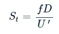
The Strouhal number is often given as
Where,
f= frequency of vortex shedding
D= characteristic diameter of the cylinder
U'= fluid flow velocity
3. Resistance coefficient:
In fluid dynamics, the drag coefficient is a dimensionless quantity that is used to quantify the resistance or resistance of an object in a fluid medium such as air or water. It is used in a drag equation in which a lower drag coefficient indicates that the object will have less aerodynamic or hydrodynamic drag. The drag coefficient is always associated with a specific area.
The drag coefficient of any object includes the effects of two fundamental contributors to fluid dynamic drag: skin friction and form drag. The drag coefficient of an airfoil or airfoil also includes the effects of lift-induced drag. The drag coefficient of a complete structure such as an aircraft also includes the effects of interference drag
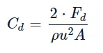
The drag coefficient Cd">Cd is defined as
where:
- Fd is the drag force, which is by definition the force component in the direction of the flow velocity,
- ρ is the mass density of the fluid,
- u is the flow speed of the object relative to the fluid,
- A is the reference area.
4. Lift coefficient:
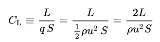
The lift coefficient is a dimensionless coefficient that gives the lift generated by a lifting body in relation to the density of the fluid around the body, the velocity of the fluid, and the associated reference area. A lifting body is a foil or a complete foil-carrying body, such as a fixed-wing aircraft. CL is a function of the body's angle to the flow, its Reynolds number, and Mach number. The section lift coefficient cl refers to the dynamic lift characteristics of a two-dimensional section of foil, with the reference surface being replaced by the strip of foil.
where
 is the lift force,
 is the relevant surface area and
q is the fluid dynamic pressure, in turn, linked to the fluid density, and to the flow speed.
Geometry: -
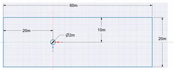
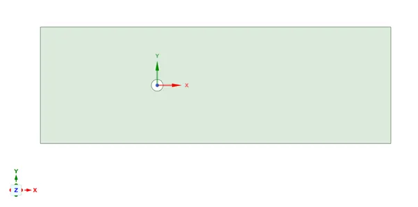
In the geometric sketch above, we see a cylinder with a diameter of 2 m, which is immersed in a liquid area of size 20 x 60 m. The entrance of the domain is 20 m to the left of the center of the cylinder, and the exit is 40 m to the right of the center of the cylinder. No thickness is provided to the geometry as this is a 2D simulation. After entering the details, the geometry will be:
Meshing:-
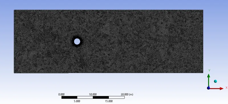
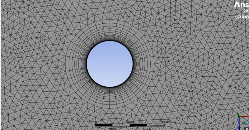
Meshing involves creating a small discrete region for calculating the governing equations. The mesh should be fine enough to compensate for any changes that occur during the simulation. The mesh size used for the stationary and unsteady solvers will be the same, which is 0.25 m for the total domain. It is important to capture the flow around the cylinder as a bout of flow separation. An inflatable layer needs to be used to capture the flow near the cylinder. The inflation creates a hexahedral mesh near the cylinder, which causes the solution to converge and provide an accurate solution.
Before creating the inflatable layer, the edge of the cylinder had to be captured using a local edge-size meshing method. Mesh size or number of layers can be used as user input for edge sizing. In this case, the mesh size 250mm. The puff layer property is the thickness of the first layer in which the height of the first layer is 0.05 and the amount of the layer is 20 to capture a larger area near the cylinder with a growth rate of 1.2 . After applying this value to the geometry, the mesh will look like this:
Then we should add inflation which is used to create body-fitted mesh
Setting up Ansys fluent
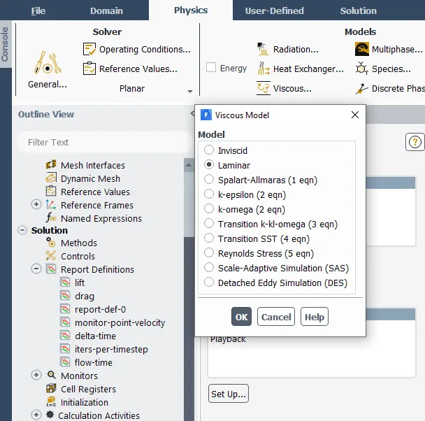
Before opening the set up we should update the mesh. Then we should change the viscous flow to laminar
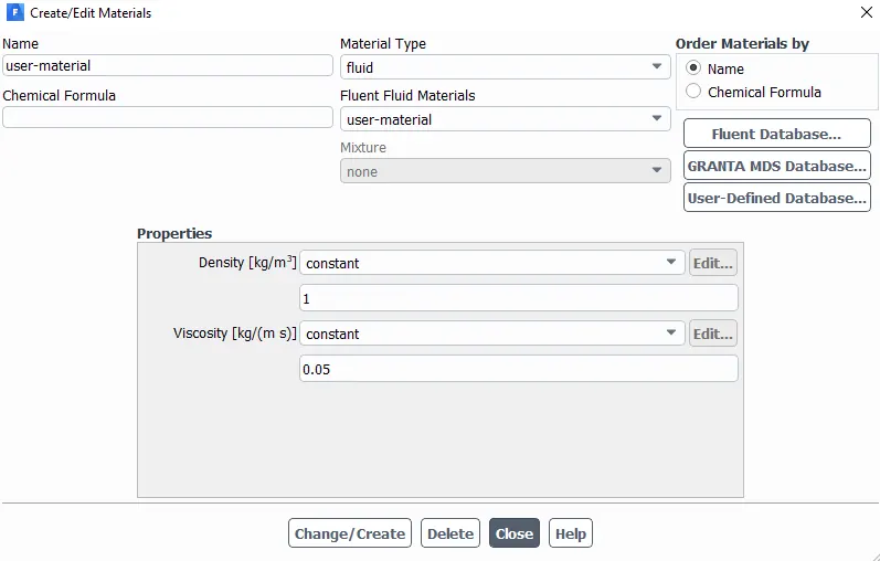
Open Materials and create a fluid that is to be used for the simulation for this case, it is air and also inputs the density and kinematic viscosity values.
Fluent details/procedure:
1. laminar model
2. fluid: Air
3. Method of discretization: Simple
4. Density/kinematic viscosity: 1/0.05
5. Creating a monitor point behind the cylinder by selecting point under surfaces in the results bar.
6. After creating the monitor point, create reports/plots for drag, lift, velocity wrt cylinder.
7. Create plots for the velocity at the monitor point to analyze the vortex shedding.
8. Use hybrid initialization for steady-state and standard for transient state simulations.
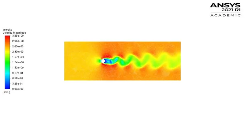
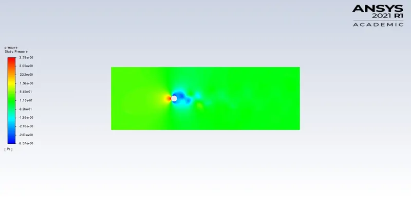
(i) Simulate the flow with the steady case and calculate the Strouhal number for Re=100 and velocity 2.5m/s.
- Velocity contours
-
- pressure contour
-
- Residuals plot
- Drag and lift coefficient
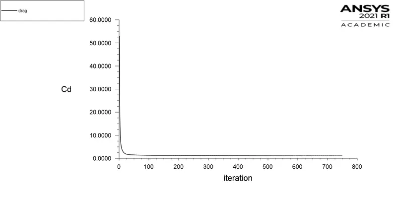
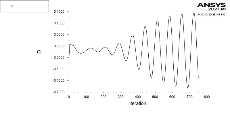
- velocity at the monitor point
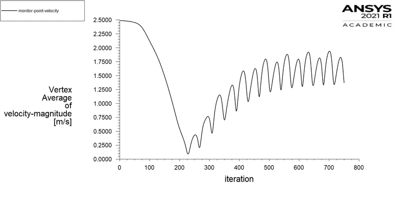
- Strouhal number plot
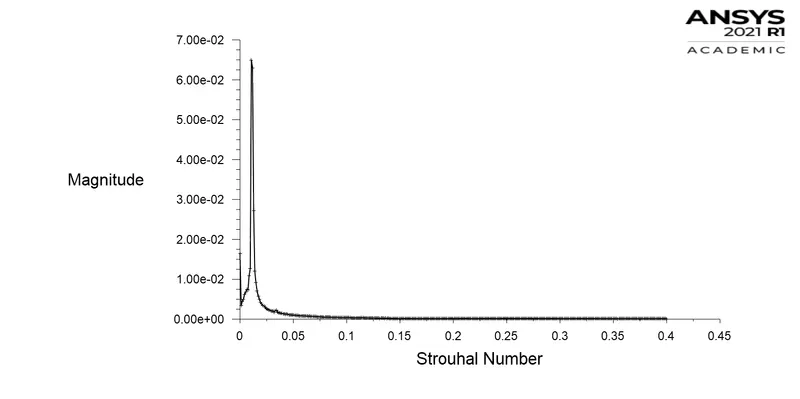
-
-
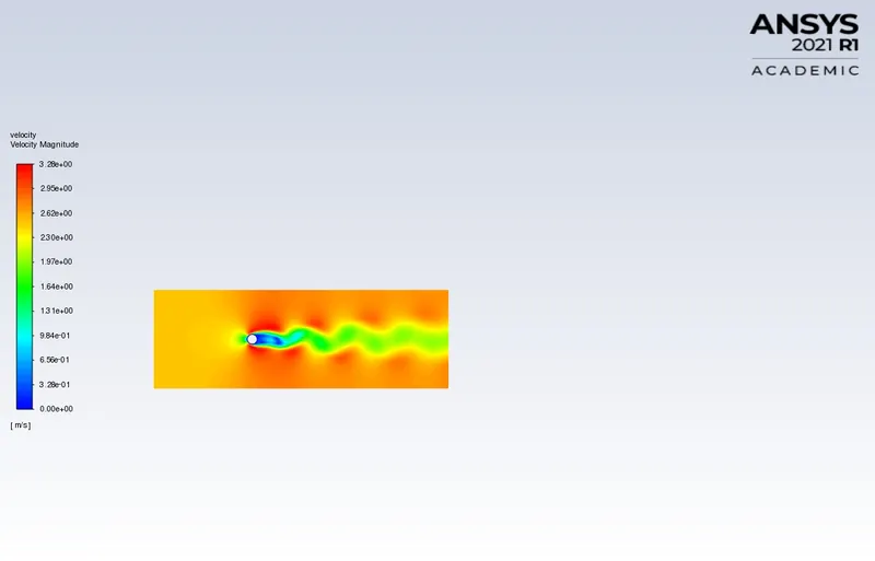
(ii) Simulate the flow with the unsteady case and calculate the Strouhal number for Re=100 and velocity 2.5m/s.
- Velocity contour
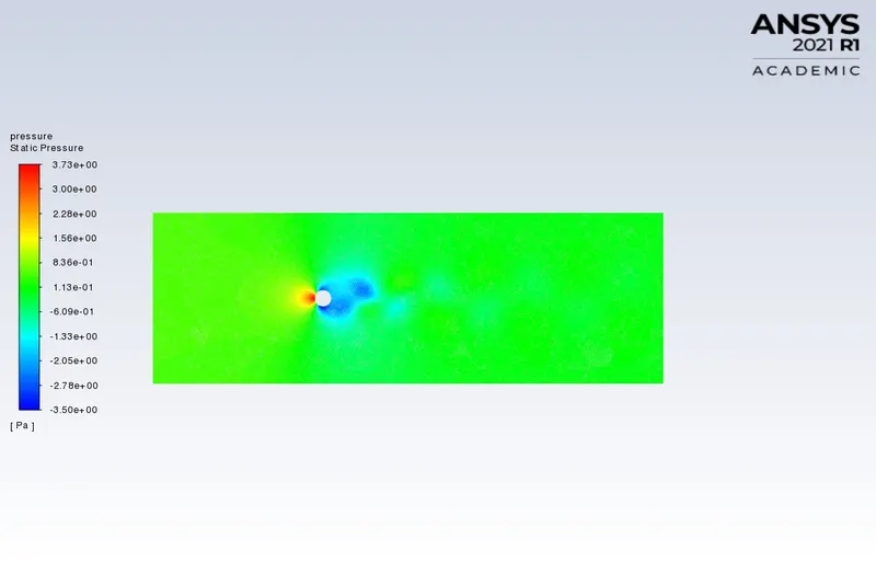
- pressure contour
-
- Residuals plot
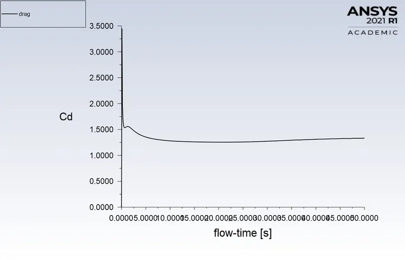
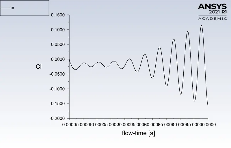
- Drag and lift coefficient
- velocity at the monitor point
- Strouhal number plot
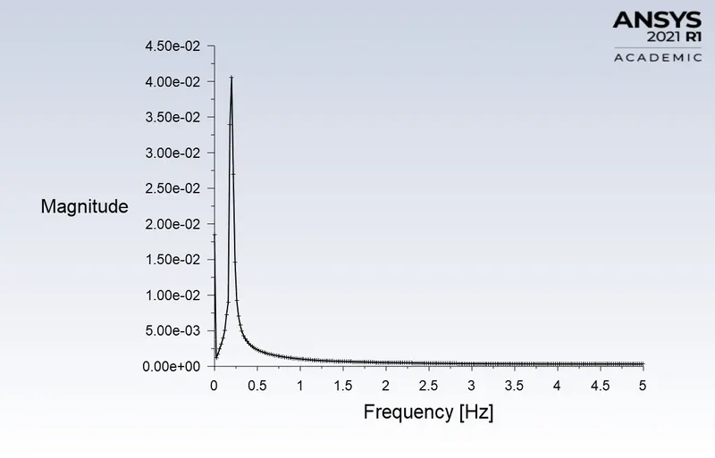
solver Cd CL Strouhal number steady-state 1.365 -0.13 0.01333 unsteady-state 1.3336 -1.179 0.1996 Part-2
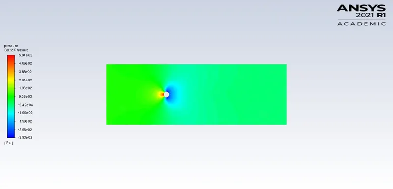
(i) Simulate the flow with the steady-state solver for Re=10.
For Re=10 velocity v=0.25m/s
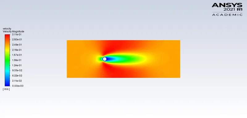
- Velocity and pressure contours
- Residuals plot
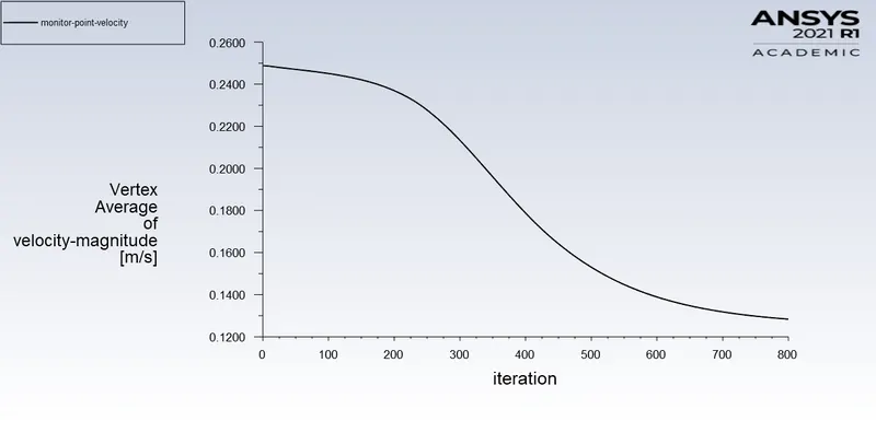
- Drag and lift coefficient
- velocity at the monitor point
(ii) Simulate the flow with the steady-state solver for Re=100.
For Re=100 velocity v=2.5m/s
- Velocity and pressure contours
- Residuals plot
- Drag and lift coefficient
- velocity at the monitor point
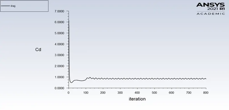
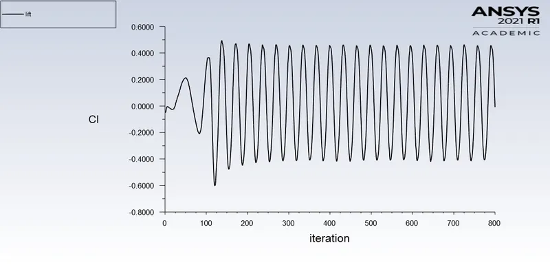
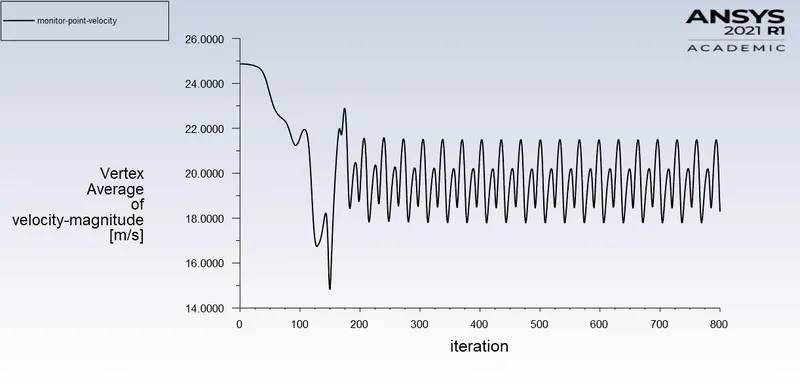
(iii) Simulate the flow with the steady-state solver for Re= 1000.
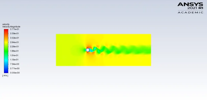
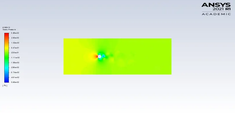
For Re=1000 velocity v=25m/s
- Velocity and pressure contours
- Residuals plot
- Drag and lift coefficient
- velocity at the monitor point
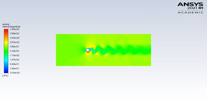
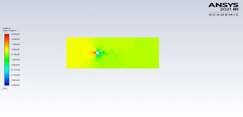
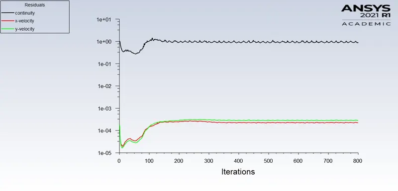
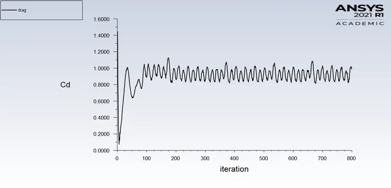
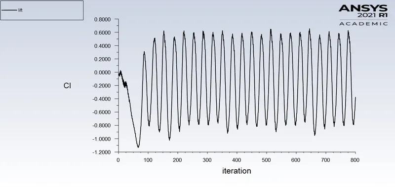
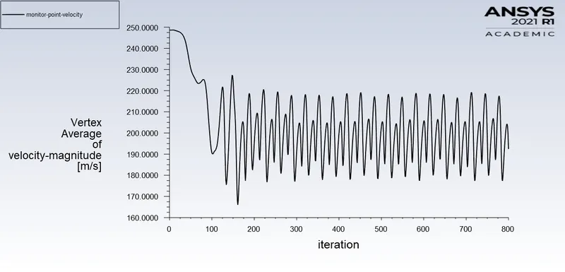
(iv) Simulate the flow with the steady-state solver for Re= 10000.
For Re=10000 velocity v=250m/s
- Velocity and pressure contours
- residual plot
- Drag and lift Coefficient
- velocity at the monitor point
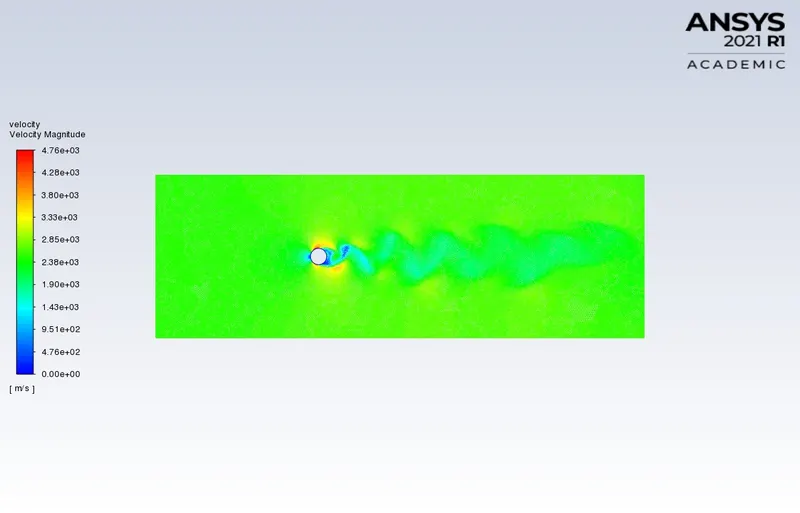
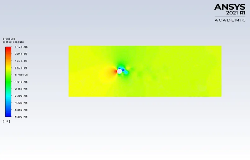
(v) Simulate the flow with the steady-state solver for Re= 100000.
For Re=100000 velocity v=2500m/s
- Velocity and pressure contours
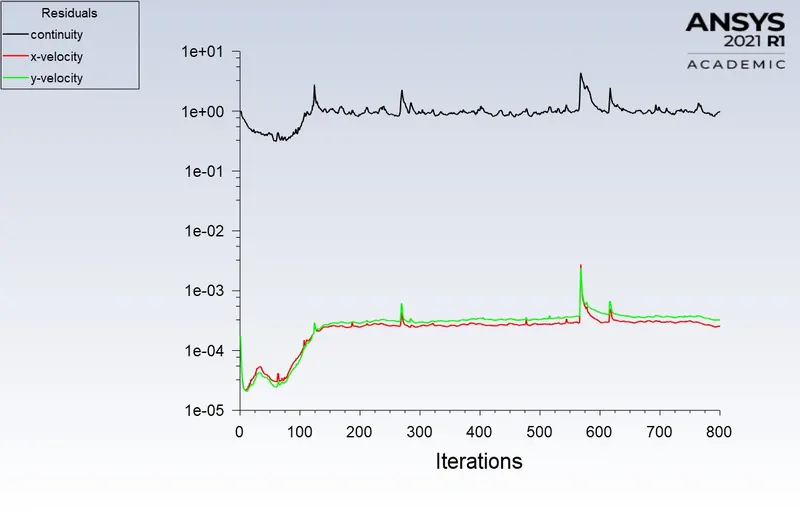
- residual plot
- Drag and lift Coefficient
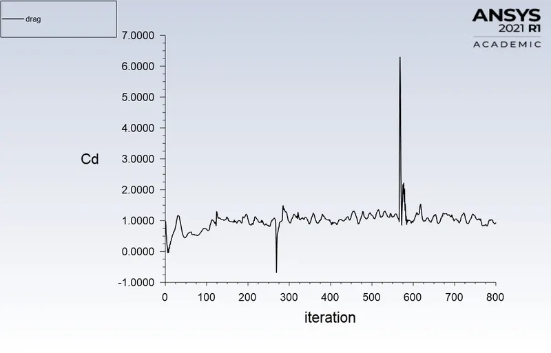
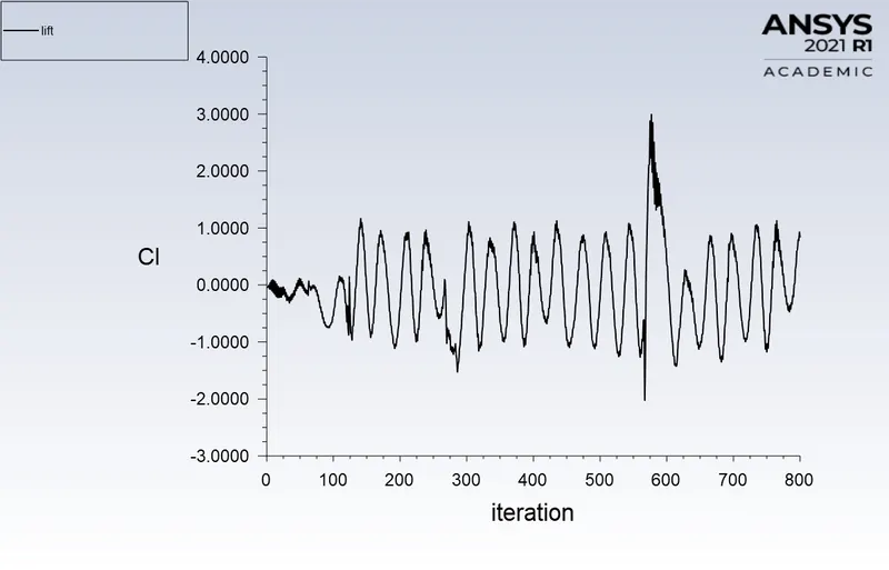
- velocity at the monitor point
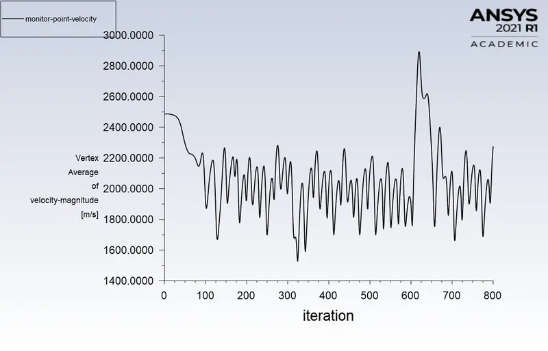
-
Result:
Drag and lift coefficient for different Reynolds number
Re Cd CL 10 3.33 -0.00155 100 1.365 -0.13 1000 0.808 -0.00839 10000 0.9876 -0.373 100000 0.937 0.833 .Error with respect to the theoretical values from the reference material,
Reynolds number theoretical Cd Numerical Cd error 10 3.5 3.333 4.77% 100 1.4 1.365 2.5%
Conclusions:
*In the first case, the flow over the cylinder is simulated for both steady and unsteady cases with Re=100 and Von Karman Vortex Street phenomena are also observed with the generated results.
*The necessary graphs are plotted to observe that the flow is converged and vortex shedding occurs.
*Contours are generated to observe the flow through the cylinder.
*By plotting the power spectral density vs. frequency, the Strouhal number is calculated.
in the second case
*six different simulations i.e. (Re = 10,100,1000,10000,100000,1000000) are simulated to observe the behavior of drag and lift coefficients by varying the Reynolds number.
*In order to observe the behavior of the drag coefficients for the simulations, the flow velocity is varied to vary the Reynolds number and the other parameters are kept constant.
*As we know, if Reynold's number is less than 2000, then the flow in the pipe is laminar. Therefore we use the viscous model = laminar.
*For Re=10, no vortex formation was observed and in the remaining cases it is clearly observed.
According to the basic conditions and parameters, the results are validated from the literature.
*As we refine the mesh, we need to run more iterations.
From the above table it can be concluded that the error percentage is less than 5%