Week 5 - Curve fitting

OBJECTIVE:

A Python codes to execute curves.

TARGET:

1. Clear codes for linear and cubic polynomial fits to Cp data.
2. To plot linear and cubic fit curves along with raw data points.
3. To measure fitness characteristics for both curves.

THEORY: Curve fitting is how we model or represent the distribution of data by fitting the best fit function (curve) along the entire range. Ideally, it will capture a trend in the data and allow us to predict how the data series will behave in the future.

Curve fitting: It is the process of formulating a mathematical function that has the best fit for the series of given data points.

Best fit means to construct a curve where the distances between the actual and the predicted values are minimum.

A perfect fit means that the error between the actual and predicted values are zero.

Assume function f(x) to satisfy the data points (x1,y1), (x2,y2).. and so on.

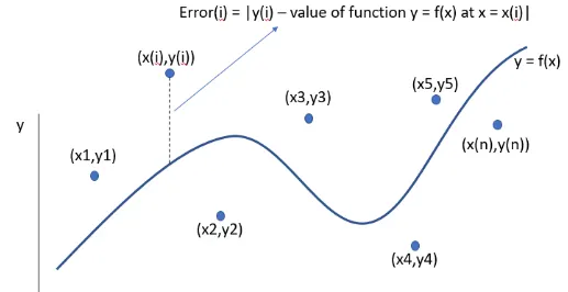
Sum of squared error = N∑i=1(y(i)−f(x(i))2

If the proposed equation is an nth degree polynomial

f(x)=A1+A2⋅x+A3⋅x2+..+A n⋅xn−1)

Curve types include:

Interpolation where you discover a function that exactly fits the data points. Since this assumes no measurement error, it has limited applicability to real-life scenarios.
Smoothing is when we find a function that approximately fits the data points, but allow room for error and allow our true points to be close but not necessarily on the line; given that the error is minimized overall.
Fitting a linear and polynomial curve:

(i) Linear curve fitting or linear regression occurs when the data is fitted to a straight line. Although your data may have some curve, a straight line provides a good fit for predictions.

Since the equation of a general straight line is always given by f(x)= a x + b, the question arises: what a and b is the best fitting line for our data?

If we consider the vertical distance from each point to the perspective line as an error and add them up within our range, we get a specific number that expresses how far it is from the "best" perspective line.

The best straight line can be considered the line that gives the minimum error.

Since we're interested in the distance from our points to the line—it doesn't matter if it's a positive or negative distance—we square the distance in our error calculations. This also allows us to weigh larger errors more heavily. This method is therefore called the method of least squares.

(ii) Polynomial curve fitting is when we fit our data to the graph of a polynomial function. The same method of least squares can be used to find the polynomial of a given degree that has the minimum total error.

To choose the best curve fit, the following four parameters help us measure the quality of the fit criteria, or how well the equations represent the given data points:

Sum of squares due to error (SSE),
R-squared (R2),
Adjusted R-squared,
root mean square error (RMSE)
GOVERNING EQUATIONS USED:

Error = ∣y(i))–value of f(x)v x(i)∣ = |y(i)−f(x(i))|,
SSE (sum of squared error) = n∑i=1Error(i)2,
SSR (regression sum of squares) = n∑i=1(f(x(i))−Mean)2,
SST (Sum of Square of Sum) = SSE+SSR ,
R2 (R squared) = SSRSST,
RMSE (root mean square error) = √SSEn,
where n is the total number of available data points.

Raw temperature (K) and specific heat (kJ/kcalK) data are obtained here

Python code:-

"""
by shiek hafeez
A program to measure fitness characteristics for the linear and cubic polynomial for the Cp data:
"""
import math
import matplotlib.pyplot as plt
import numpy as np
from scipy.optimize import curve_fit

# Curve fit function
# Linear function
def function_0(t,a,b):
	return a*t + b 
# Cubic function	
def function_2(t,a,b,c,d):
	return a*pow(t,3) + b*pow(t,2) + c*t +d
	

# Reading thermodynamic data file
def read_file():
	temperature = []
	cp = []
	for line in open('data','r'):
		values = line.split(',')
		temperature.append(float(values[0]))
		cp.append(float(values[1]))

	return [temperature , cp]

# Main Program
temperature , cp = read_file()

#linear curve fitting
popt, pcov = curve_fit(function_0,temperature,cp)
fit_cp_l = function_0(np.array(temperature), *popt)
plt.figure(1)
plt.plot(temperature,cp,color="blue",linewidth=3)
plt.plot(temperature,fit_cp_l,color='red',linewidth =2)
plt.legend(['Actual data','Curve fit'])
plt.xlabel('Temperature (K)')
plt.ylabel('Cp')
plt.title('Linear Curve fitting')
plt.show()

#cubic curve fitting
popt, pcov = curve_fit(function_2,temperature,cp)
fit_cp_c = function_2(np.array(temperature), *popt)
plt.figure(2)
plt.plot(temperature,cp,color="blue",linewidth=3)
plt.plot(temperature,fit_cp_c,color='red',linewidth = 2)
plt.legend(['Actual data','Curve fit'])
plt.xlabel('Temperature (K)')
plt.ylabel('Cp')
plt.title('Cubic Curve fitting')
plt.show()

''' 
Measuring the fitness characetristics of the curves 

 SSE (sum of error squared)
 SSR (sum of squares of the regression)
 SST = SSE + SSR
 R^2 = SSR/SST
 RMSE = (SSE/l)^0.5

 Finding mean of Cp data
 mean = ( sum of all elements)/(total number of elements)
 '''

s = np.sum(cp)
l = np.size(cp)
m = s/l
print('Mean of all cp :',m)
print('')
# For Linear curve fit

linear_sse = 0
linear_ssr = 0
for i in range(l):
    linear_error = abs((np.sum((cp[i] - fit_cp_l[i]))))
    linear_sse = linear_sse+pow(linear_error,2)
    linear_ssr = linear_ssr+ np.sum(pow((fit_cp_l[i] - m),2))

 
linear_sst = linear_sse + linear_ssr
print('linear_sst :',linear_sst)
linear_R2 = linear_ssr/linear_sst
print('linear_R2 :',linear_R2)
linear_rmse = pow((linear_sse/l),0.5)
print('linear_RMSE :',linear_rmse)
print('')


# For Cubic curve fit
cubic_sse = 0
cubic_ssr = 0
for j in range(l):
    cubic_error = abs(np.sum((cp[i] - fit_cp_c[i])))
    cubic_sse = cubic_sse+(pow(cubic_error,2))
    cubic_ssr = cubic_ssr+np.sum(pow((fit_cp_c[i] - m),2))

 
cubic_sst = cubic_sse + cubic_ssr
print('cubic_sst :',cubic_sst)
cubic_R2= cubic_ssr/cubic_sst
print('cubic_R2 :',cubic_R2)
cubic_rmse = pow((cubic_sse/l),0.5)
print('cubic_RMSE :',cubic_rmse)

#splitwise method

import numpy as np
import matplotlib.pyplot as plt
from scipy.optimize import curve_fit
from statistics import mean 
	

def fitcubic(T,a,b,c,d): #Cubic fit equation
	return a*pow(T,3)+b*pow(T,2)+c*T+d

def read_file(): #Function to open and read values from file 'data'
	t = [] #array temperature
	cp = [] #array specific heat for constant pressure
	for line in open('data','r'): #open file data in read mode 
		value = line.split(',') #delimiter ','
		t.append(float(value[0])) 
		cp.append(float(value[1]))

	return[t,cp]

t, cp = read_file() 

t1 = np.array(t[0:800])
t2 = np.array(t[800:1600])
t3 = np.array(t[1600:2400])
t4 = np.array(t[2400:3200])


popt1, pcov1 = curve_fit(fitcubic, t1, cp[0:800]) 
fit_values = []
fit_values = fitcubic(np.array(t1), *popt1)


popt2, pcov2 = curve_fit(fitcubic, t2, cp[800:1600])
fit_values = np.append(fit_values,(fitcubic(np.array(t2), *popt2)))

popt3, pcov3 = curve_fit(fitcubic, t3, cp[1600:2400])
fit_values = np.append(fit_values,(fitcubic(np.array(t3), *popt3)))

popt4, pcov4 = curve_fit(fitcubic, t4, cp[2400:3200])
fit_values = np.append(fit_values,(fitcubic(np.array(t4), *popt4)))

#R squared
SSE = sum(pow((cp-fit_values),2)); #sum of the squared error
SSR = sum(pow(fit_values-mean(cp),2)); #sum of the square of the regression
SST = SSE+SSR;
R_sq = SSR/SST;#R squared calculation
print('R squared for a splitwise fit = ',R_sq)

plt.plot(t,cp,'r')
plt.plot(t,fit_values,'b')
plt.xlabel('Temperature (K)')
plt.ylabel('Cp')
plt.legend(['actual','curve fit'])
plt.title('splitwise fit')
plt.show()

SOLUTION STEPS:

1. First, necessary modules like math, matplotlib, NumPy, scipy are imported to perform their respective functions.
2. Two functions are defined that return linear and cubic equations.
3. The following data is read into Python by placing it in the correct directory and creating a read_file function. A For loop is used to run each line using the 'open' command with 'r' to read it.
Two individual column matrices of temperature and specific heat are derived 4. from the obtained data.
5. For curve approximation, 'popt' and 'pcov' are used as output to store the parameters obtained by the 'curve_fit' command, which takes input as the desired function (linear or cubic), temperature and Cp. Now another variable named 'fit_cp' stores the new Cp values ​​calculated using the temperature field.
6. Both raw data sets and predicted data sets are plotted and compared to find fitness characteristics for both linear and cubic polynomial curves.
Various parameters such as SSE, SSR, SST, R2, RMSE are calculated to measure the fitness characteristics for both curves. 7.A plot that has the highest R2 or closest to 1 is considered suitable.

RESULTS :

• The following are the output of the above program-
• 

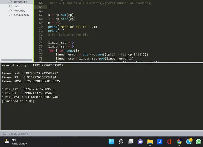
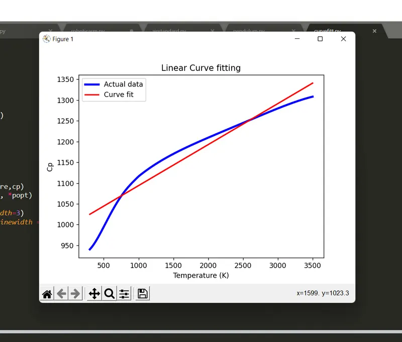
• For Linear Curve fitting the plot obtained is-
• 

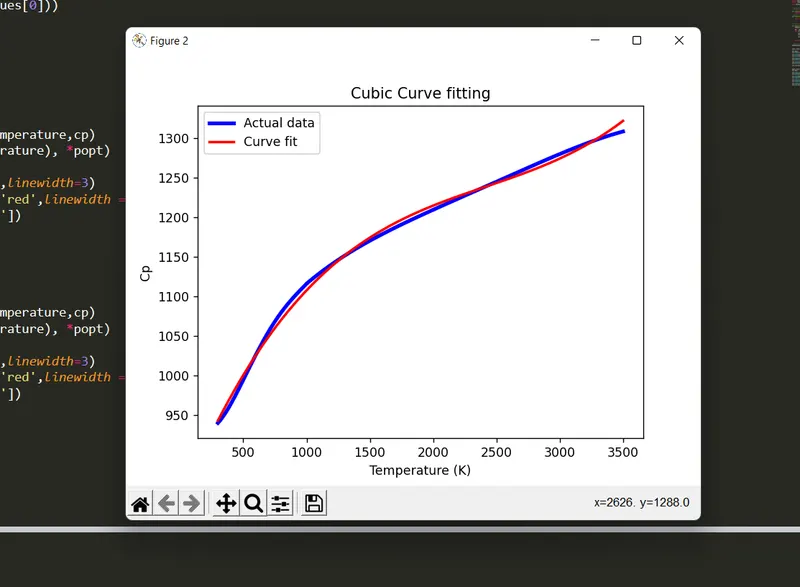
• For Cubic Curve fitting the plot obtained is-
• 

Based on the above work, we can answer the following questions:

Q. What do pop and pcov mean?

Ans. 'popt' represents a matrix that stores and extracts the coefficients for interpolation functions according to the defined general equations.

popt : array, Optimal values ​​for the parameters to minimize the sum of squares of the residuals f(xdata, *popt) - ydata

'pcov' represents a square matrix that stores the estimated covariance values ​​of the coefficients above. The diagonal elements of this square matrix also represent the variance of these coefficients.

pcov: 2d field

Estimated covariance pop. The diagonals give the variance of the parameter estimate. To calculate one standard deviation of the parameters, use perr = np.sqrt(np.diag(pcov)). How the sigma parameter affects the estimated covariance depends on the absolute_sigma argument, as if True, sigma is used in an absolute sense and the estimated covariance parameter pcov reflects these absolute values. If False, only the relative magnitudes of the sigma values ​​matter. The returned covariance matrix pcov is based on scaling sigma by a constant factor.

Question: What does np.array(temperature) do?

Ans This command converts each temperature value in the data file to an array using the NumPy module.

Question: What does the * in *popt mean?

Ans '*' , '*popt' indicates and returns each coefficient stored in the popt field.

Q: What needs to be done to make the curve fit perfectly?

Ans:If we increase the order of the polynomial, the error produced will be less and the curve will fit perfectly. As the order of the polynomial increases, the value of R2 will approach 1 and is assumed to be a perfect fit.

Conclusion:

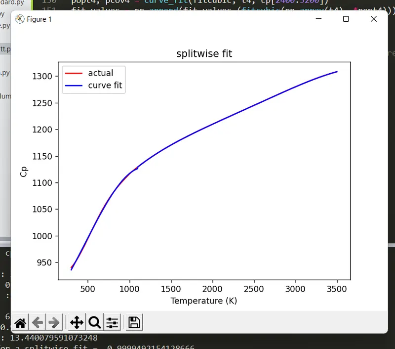
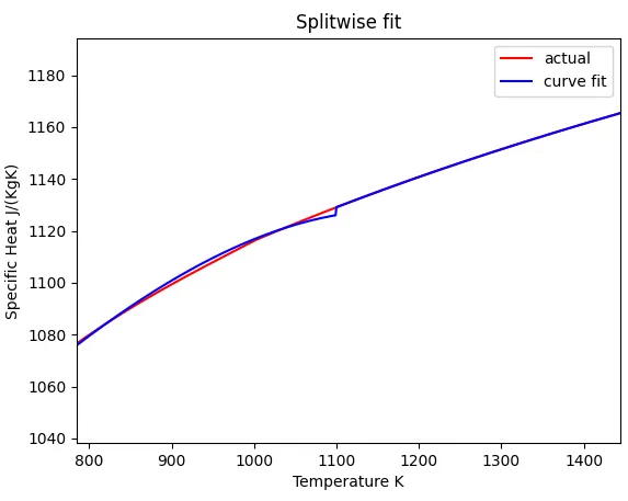
By observing the square of the R value for each fit, we can say that the splitwise method with the cubic function provides the best fit for the given data set, while the linear function provides the worst fit.