Week 9 - FVM Literature Review

TO EXPLAIN THE NEED FOR THE INTERPOLATION SCHEMES AND FLUX LIMITER IN THE FVM(FINITE VOLUME METHOD).

Aim:

To describe the need for the interpolation schemes in the FVM and flux limiter.

METHOD OF THE CFD:

To solve a real-world problem, people discover three simple schemes for numerical solutions

• Finite difference method
• Finite Element Method
• Finite volume method
• Finite difference method:

Finite Difference Method:

This method solves the equation, i.e. dividing it into individual points or nodes. This method involves solving discretizations using a differential equation.

Finite Element Method:

This method involves dividing the domain into wish elements. By solving an element in the system. Finite element analysis is a special method for solving two or three dimensional problems.

Finite volume method:

The finite volume method (FVM) is a method for representing and evaluating partial differential equations in the form of algebraic equations. In the finite volume method, volume integrals in a partial differential equation that contain a divergence term are converted to area integrals using the divergence theorem. These terms are then evaluated as fluxes on the surfaces of each finite volume. Because the flow entering a given volume is the same as the flow leaving an adjacent volume, these methods are conservative. Another advantage of the finite volume method is that it is easily formulated to allow the use of unstructured meshes. The method is used in many computational fluid dynamics packages. "Final volume" refers to the small volume surrounding each node point on the network.

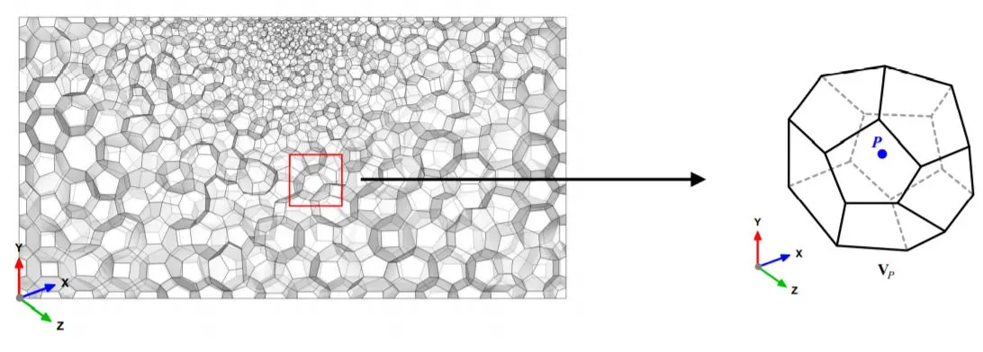
Interpolation schemes in the finite volume method (FVM):

The interpolation schemes used in the FVM method are as follows

• Upwind interpolation scheme. (UDS)
• Central difference approximation. (CDS)
• Quadratic upwind differentiation scheme. (QUICK)
• Hybrid interpolation scheme. (CDS and UDS)
• Schematic of reduction of total deviation. (TVD)

1. Upwind Interpolation Scheme(UDS):

In this scheme we use the node in the upwind or upstream of the given node. It is generally used for convection dominated problems (i.e Pe>1). ,

``{(2x,+,17y,=,23),(x,-,y,=,5):}``

The values for this at the interface is given by

for`v > 0 ; u i − 1 2 ≈ u i − 1 ; u i + 1 2 ≈ u i`

`I c ≈ v u i − u i − 1 Δ x` Backward differencing scheme

`For v > 0 ; u i − 1 2 ≈ u i − 1 ; u i + 1 2 ≈ u i` Forward differencing scheme

2.Central Differencing Approximation (CDS):

Approximate values ​​of the variable at the center of the control volume (CV) surface by linear interpolation of the values ​​at the two nearest calculation nodes.

`f e = f E λ e + f p ( 1 − λ e )`where`λ e = frac{x e − x p}{ x E − x P}`

Linear interpolation is equivalent to using the central difference formula of the first-order derivative, and therefore this scheme is also called a central difference scheme (CDS).

3. Interpolation Polynomial:

`p 1 ( x ) = u L . frac{x R − x}{ x r + x} + u R .frac{ x − x L}{ x R − x L}`

The interface values are given by:

`underset (i − 1/ 2)(u) ≈ u i − 1 + u i 2`and `underset( i + 1/ 2)(u) ≈ u i + u i + 1 2`

`I c ≈ v . u i + 1 − u i − 1 2 Δ x` central differencing scheme

Taylor Series Approximation Polynomial:

The approximation is second order precise. It is the simplest and most widely used interpolation technique for the evaluation of gradients required to measure diffusive fluxes

FLOW LIMITERS:

Flow restrictors are used in numerical schemes to solve fluid dynamics problems described by highly coupled nonlinear partial differential equations. If we tend to use low-order numerical schemes to solve the governing equations, then we might get a highly oscillatory and unstable solution near the discontinuity, if present. Whereas if we tend to use higher order numerical schemes to capture the phenomenon more accurately, we tend to waste computing power. The main idea of ​​using flux limiters is to limit the spatial derivative terms near the discontinuities to physically real values ​​so that physical consistency is preserved. There are several types of flow/slope restrictor functions. They come in handy when sharp waves/peaks are present. For smoothly varying wavelets/functions, flux limiters do not work and spatial derivatives can be represented normally.

It is imperative to note that flow restrictors are also referred to as slope restrictors because both have the same mathematical form and both have the effect of limiting the gradient of the solution near shocks or discontinuities.

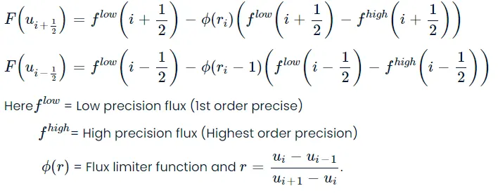
Where

flow=low resolution flux,

fhigh=high resolution flux,

ϕ(r)=flux limiter function.

where r represents the ratio of successive gradients on the solution mesh,

When the limiter equals to zero, the flux represents the low resolution scheme.

When the limiter equals to 1, the flux represents the high-resolution scheme.

There are many limiters having distinguished characters and are selected according to the problem. There is no particular limiter found to work well for all and it is selected by the trail and error method.