Week 8 - Simulating Cyclone separator with Discrete Phase Modelling

AIM : To perform analysis on cyclone separator and calculate the separation efficiency and pressure drop.  

OBJECTIVE : 

- To write a few words about any four empirical models used to calculate the cyclone separator efficiency. 

- To perform an analysis on a given cyclone separator model by varying the particle diameter from 1 μm to  10 μm and calculate the separation efficiency in each case. Discuss the results. [Using velocity as 3m/sec].

- To perform an analysis on a  given cyclone separator model by varying the velocity from 1 m/sec to 5 m/sec and calculate the separation efficiency and pressure drop in each case. Discuss the results. [Use particle diameter size as 5 μm].

THEORY:

Cyclone separator:
Cyclone separators or simply cyclones are separation devices (dry scrubbers) that use the principle of inertia to remove solid particles from flue gas. Cyclone separators are one of many air pollution control devices known as pre-cleaners because they generally remove larger pieces of particulate matter. This prevents finer filtration methods from having to deal with larger, more abrasive particles later.

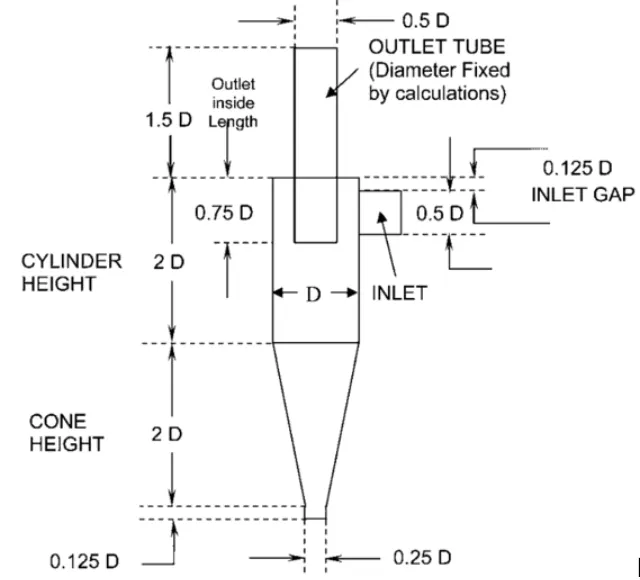
It is important to note that cyclones can vary drastically in size. The size of the cyclone depends largely on how much flue gas needs to be filtered, so larger operations usually require larger cyclones. For example, there may be several different models of one type of cyclone, and they may range in size from a relatively small 1.2-1.5 meters in height (about 4-5 feet) to around 9 meters (30 feet) - which is about as tall three-story building.

     

     

WORKING :

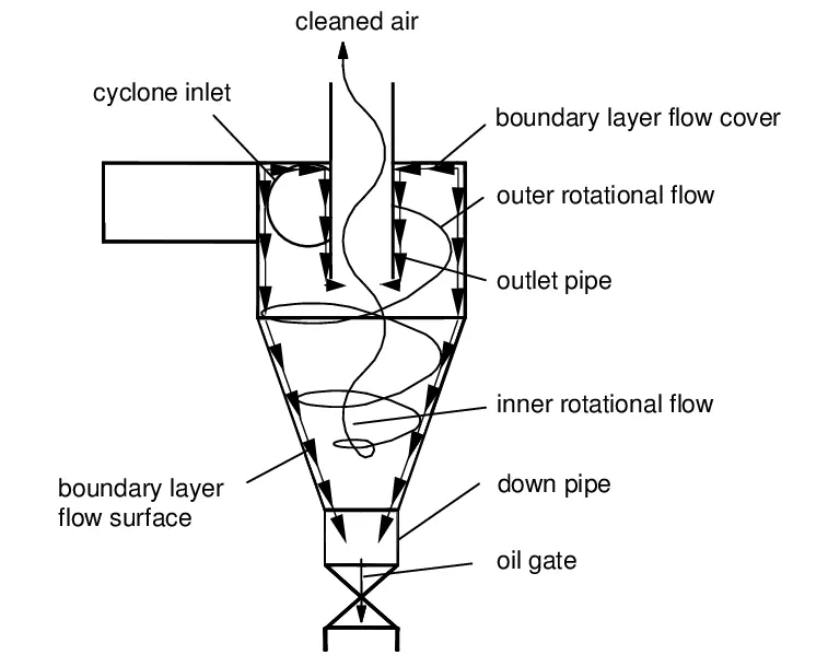
Cyclone separators work similarly to centrifuges, but with a continuous supply of dirty air. In the cyclone separator, the polluted flue gases are fed into the chamber. The inside of the chamber creates a spiral vortex, similar to a tornado. The lighter components of this gas have less inertia, making it easier for them to influence the vortex and travel up it. Conversely, larger particle components have greater inertia and are not as easily affected by the vortex.

Because these larger particles have difficulty following the high-speed spiral gas movement and eddy, the particles strike the inner walls of the vessel and fall down into the collection hopper. These chambers are shaped like an inverted cone to encourage the collection of these particles at the bottom of the container. Cleaned flue gases escape from the upper part of the chamber.

Four empirical models used to calculate cyclone separator efficiency:

1. The Iozia and Leith model:

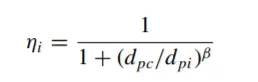
Iozia and Leith's logistic model is a modified version of Barth's model, which is developed on the basis of balance of power. The model assumes that the particle carried by the vortex endures the influence of two forces: the centrifugal force Z and the flow resistance W. The collection efficiency ηi of the particle diameter dpi can be calculated from

β is an expression for slope parameter derived based on the statistical analysis of experimental data of a cyclone with D = 170 0.25 m given as

  

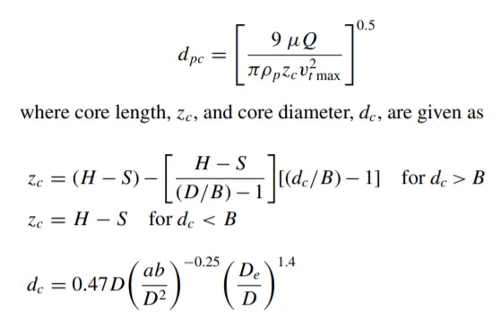
and dpc is the 50% cut size given by Barth

 

2. Li and Wang model:

Li and Wang's model includes particle reflection or reentrainment and turbulent diffusion in the cyclone wall. A two-dimensional analytical representation of the particle distribution in the cyclone is obtained. Li and Wang's model was developed based on the following assumptions:

The radial particle velocity and radial concentration profile are not constant for uncollected particles in the cyclone.
The boundary conditions considering the coefficient of turbulent diffusion and back-entrainment of particle reflection on the cyclone wall are:

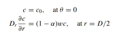
• The tangential velocity is related to the radius of cyclone by: uRⁿ = constant.

The concentration distribution in a cyclone is given as:

    

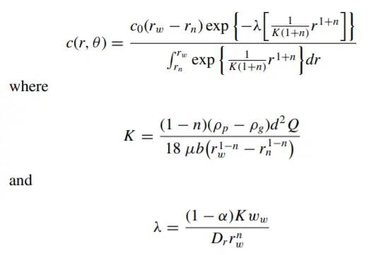
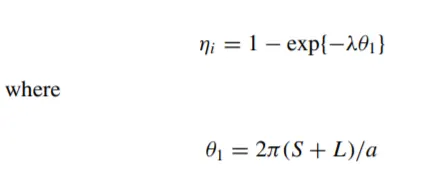
The resultant expression of the collection efficiency for particle of any size is given as

      

3. Koch's and Licht's model

The collection theory of Koch and Licht recognized the inherently turbulent nature of cyclones and the distribution of gas residence times within the cyclone. Koch and Licht described the movement of particles in the inlet and collection regions with the following additional assumptions:

The tangential velocity of the particle is equal to the tangential velocity of the gas flow, i.e. there is no slip in the tangential direction between the particle and the gas.
The tangential velocity is related to the cyclone radius according to: uRn = constant.
The force balance and particle collection equations give the degree of efficiency ηi

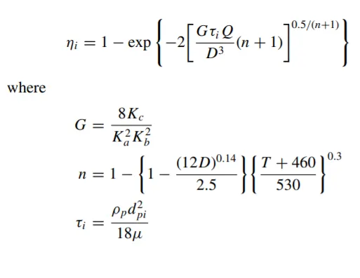
G is a factor related to the configuration of the cyclone, n is related to the vortex and τ is the relaxation term.

4. The Lapple model

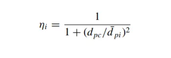
The Lapple model was developed based on a force balance without considering flow resistance. Lapple assumed that the particles entering the cyclone were uniformly distributed across the inlet opening. Particles that move from the inlet half-width to the wall in the cyclone are collected at 50% efficiency. A semi-empirical relationship developed by Lapple [1] to calculate the 50% cut diameter, dpc, is

    

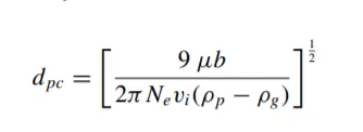
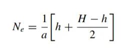
where N_e is the number of revolutions     

     

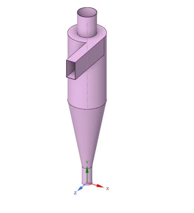
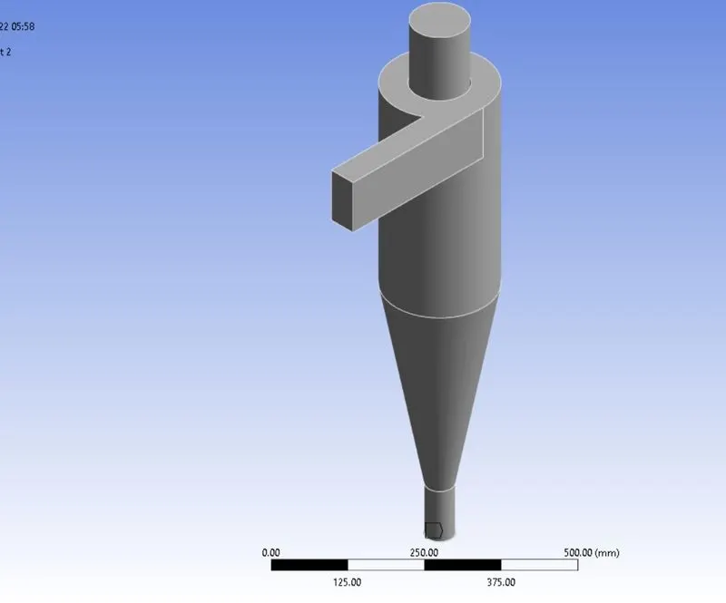
 Step1:Geometry creation

 

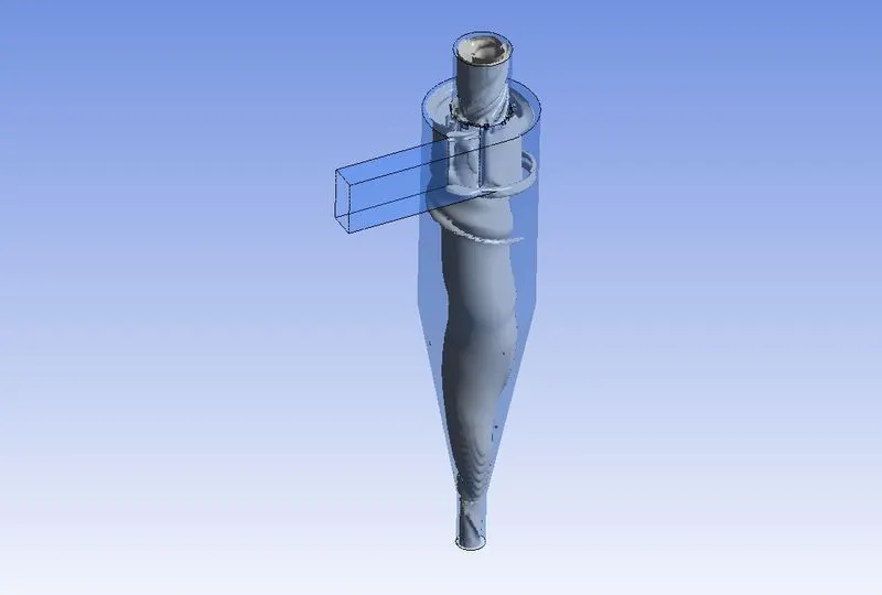
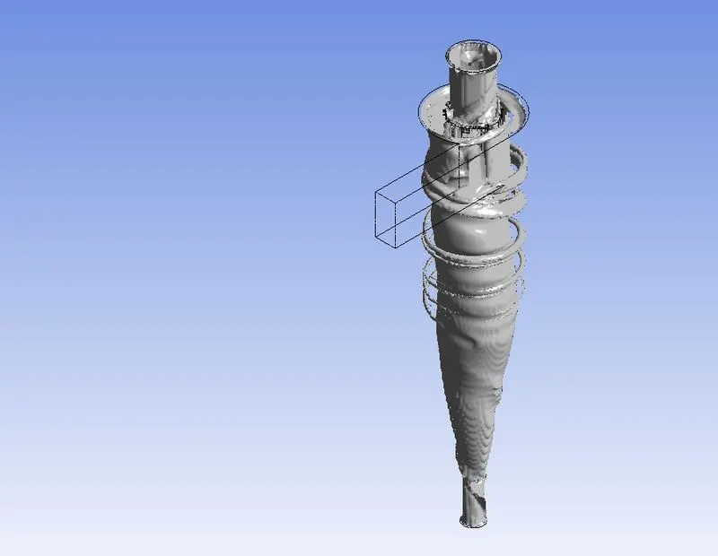
    Solid model:

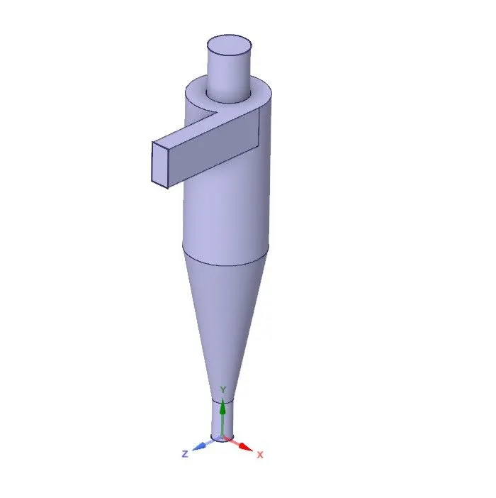
 Fluid volume:

 

 STEP 2 :  MESHING

Method:Body fitted cartesian

Number of nodes : 456604

Number of elements : 427871

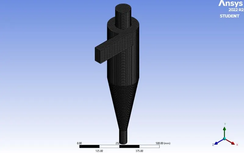
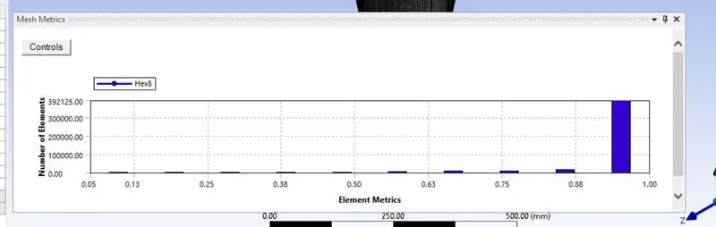
  Mesh Quality

  

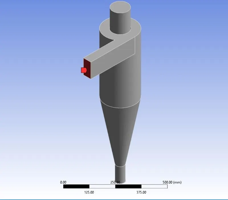
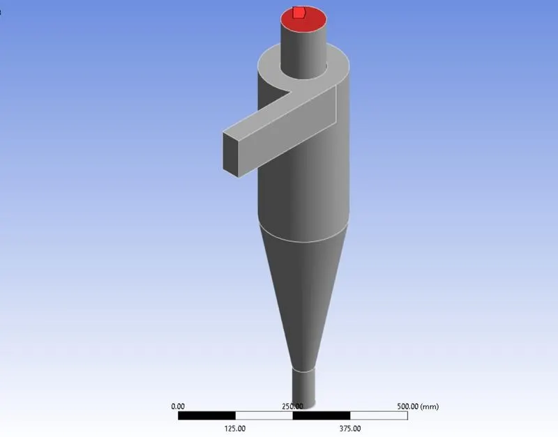
 Boundaries

  Inlet :

Outlet 1  :

 

 Outlet 2 :

 

The efficiency of collection of any size of particle is given by

            

STEP 3: SETUP AND SOLUTION

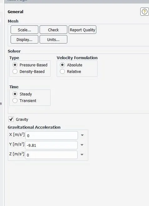
1. In this problem, the maximum speed attained by the particles and air is very less compared to the speed of sound.
   So the Mach number is <<< 0.3. Therefore, a pressure-based solver was used, as density-based solvers are generally used for simulations with Mach number > 0.3.
2. In this particular simulation, a steady-state solver was used because we do not need to observe every particle at every instant.
3. Observing the number of trapped, escaped and incomplete particles is our main motive
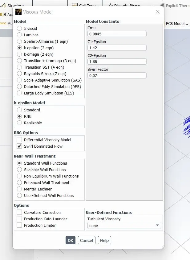
   Additionally, a gravity value of 9.81 m/s^2 in the -ve Y direction was added.
4. In this particular problem, the K-epsilon RNG model was used.
5. This model is an upgrade of the standard k-epsilon model and is mainly used for eddy flow.
6. Additionally, the "swirl Dominoval flow" option was turned on for this simulation.
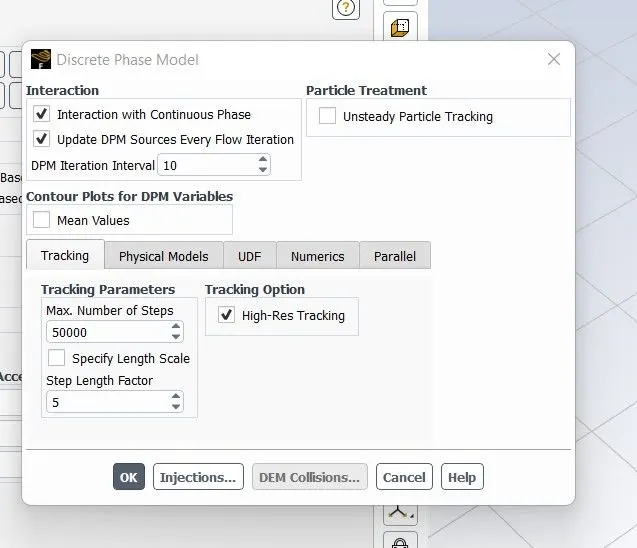
7. Then the discrete phase model option was turned on and the settings were changed.
8. Here, air particles represent the continuous phase, while solid particles represent the discontinuous phase.
9. The two phases can exchange mass and momentum in the flow.
   Coupled Flow – Discrete phase can influence continuous phase flow
   Uncoupled Flow – The discrete phase will have no interaction with the continuous phase
   In this particular case, the particle size is very small, it doesn't matter which option we chose.
   The DPM interval was chosen as 10, so the particle tracking data will be updated and displayed on the console every 10 iterations.
10. The tracking and specify length scale parameters were set as defaults.
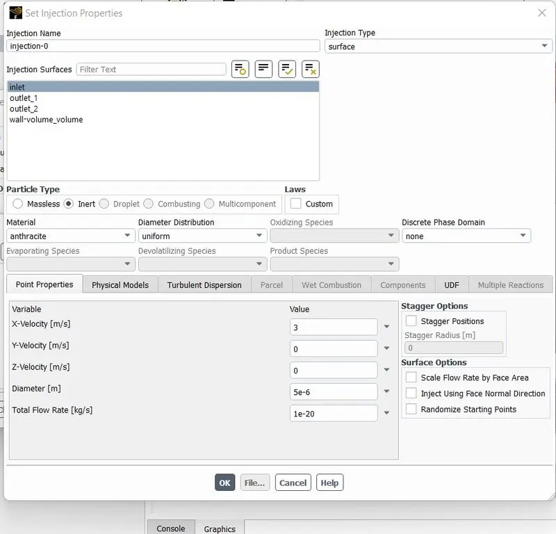
11. Then a new injection was created with the following parameters –
    Material – anthracite
    Particle type – inert
    Average distribution – uniform
    Injection type - surface
    Release from - ENTRY
    Speed ​​– 1,3,5 m/s in x direction
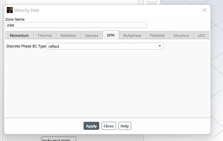
    Particle diameter – 1,3,5 microns
12. Furthermore, the boundary conditions for DPM were set accordingly
       Input - Reflect
       Wall - Reflect
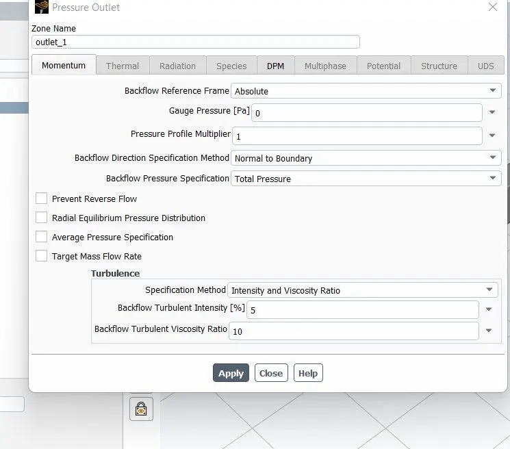
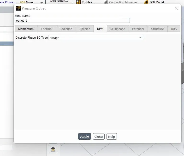
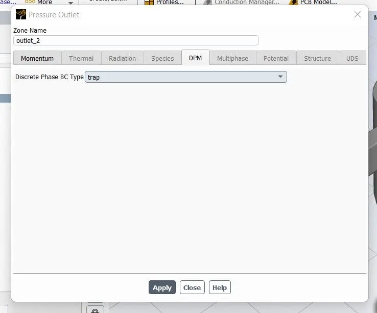
       Top of outlet - escape
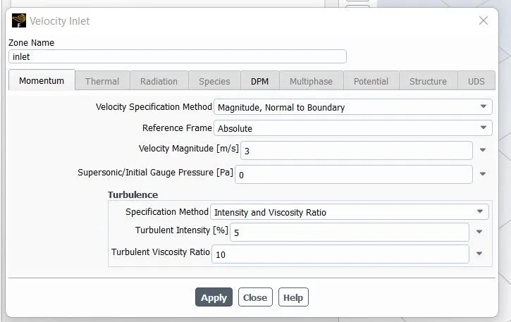
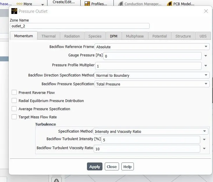
       Outlet Bottom - a trap
13. The input was set to velocity input and the output to pressure output
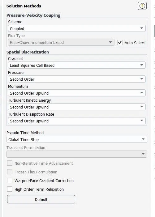
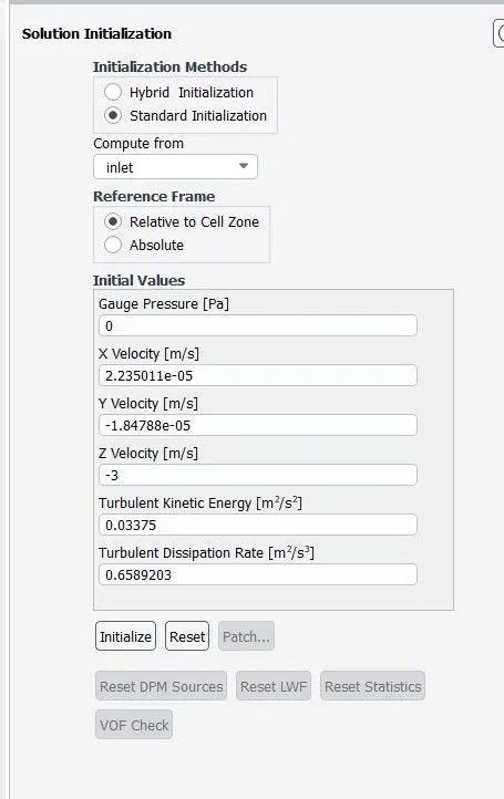
    A "second-order upwind" coupled scheme was used for turbulent kinetic energy and turbulent dissipation rate.
14. The solution was initialized using standard initialization and computed from the input.
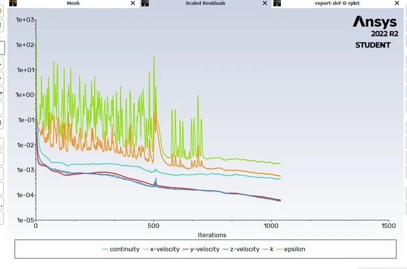
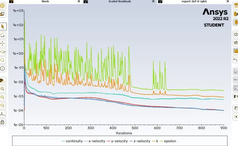
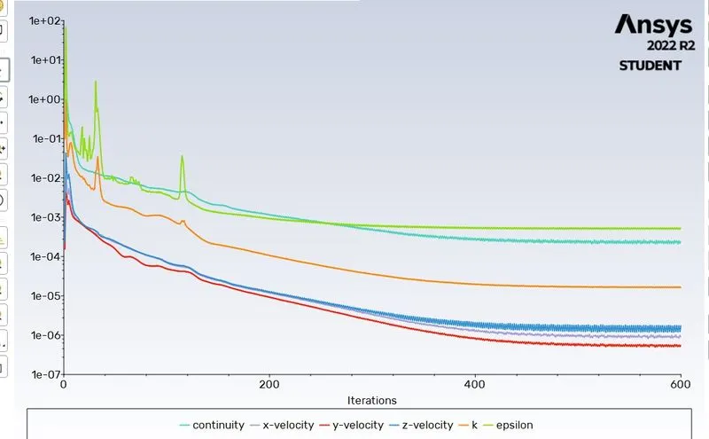
15. The problem was then run for 600 iterations and the results observed\

 

 

 

 

 

STEP 4 : RESULTS 

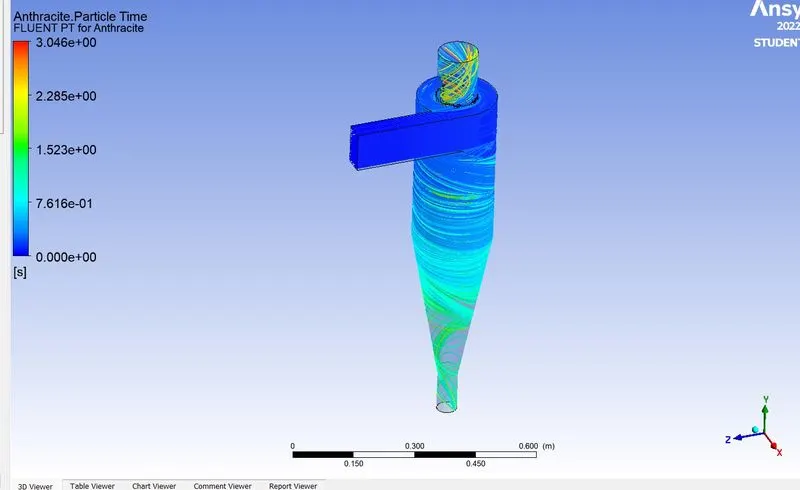
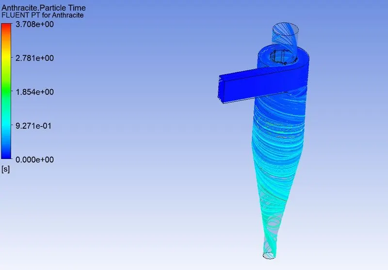
 1.Velocity = 3m/s, size = 5microns                                                            

    

 

 

 

 2.Velocity=3m/s,Size=3microns

 

 

 

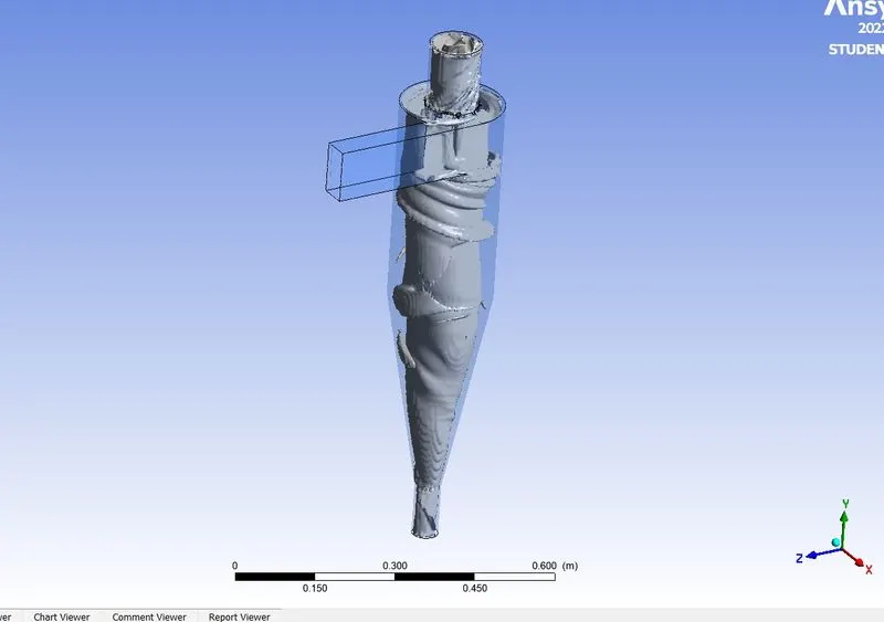
 3.Velocity=3m/s,Size=1 micron

 

 

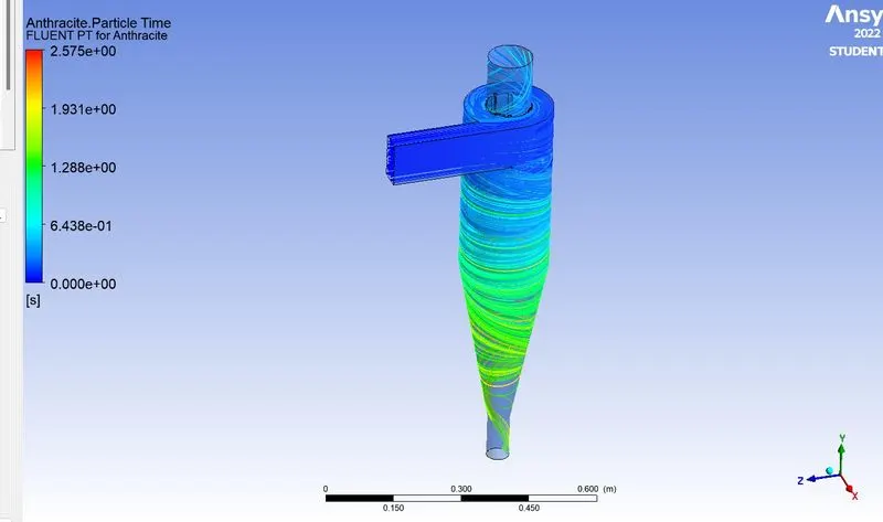
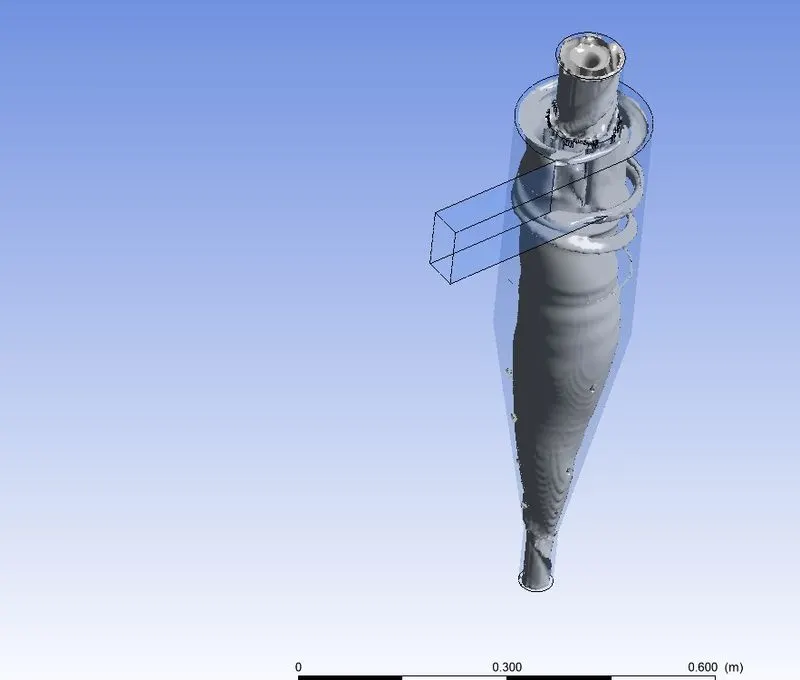
 4.Velocity=5m/s,Size=5microns

 

 

 

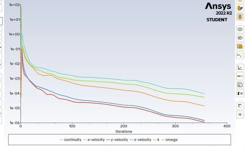
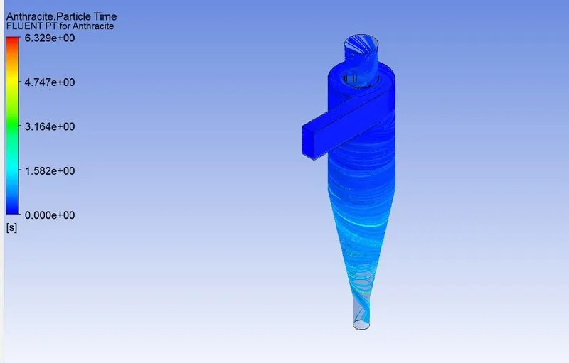
 5.Velocity=3m/s,Size=5microns

 

 

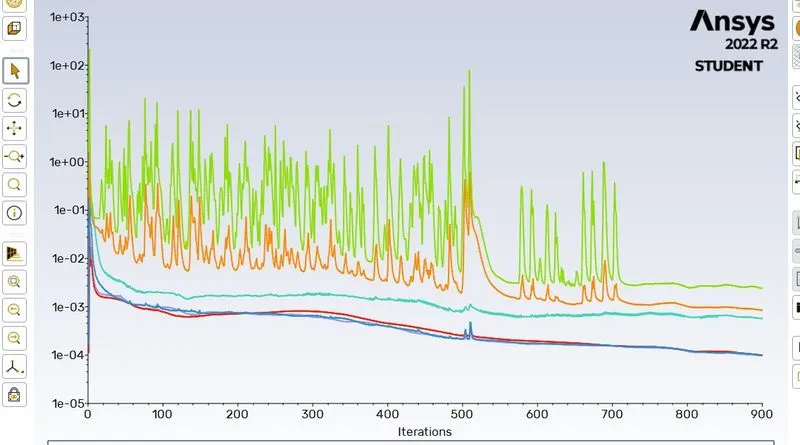
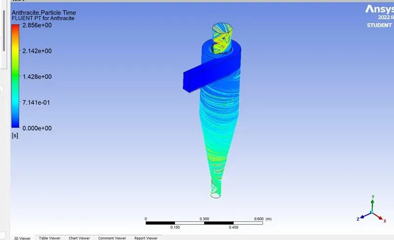
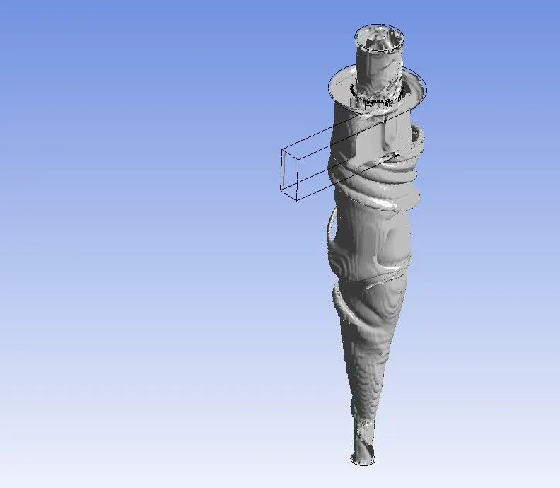
 6.Velocity=1m/s,Size=5 microns

 

 

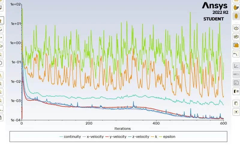
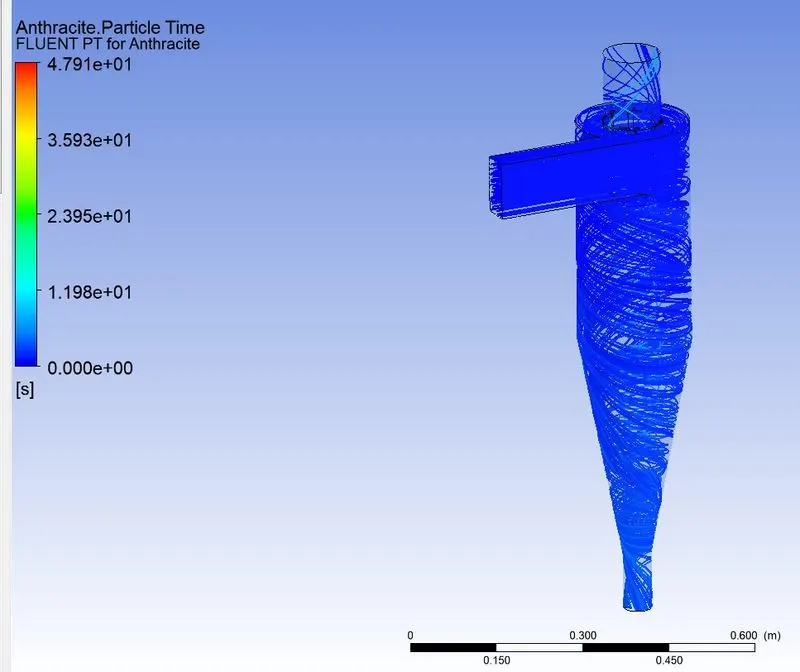
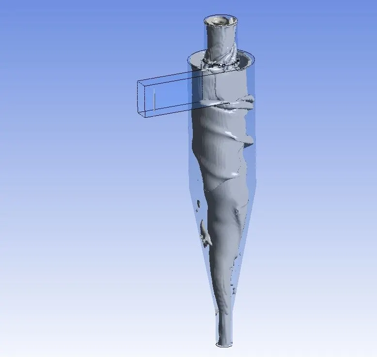
 Tables of all cases:

	Velocity and diameter	Tracked	Escaped	Trapped	Incomplete	Collector Efficiency	pressure     drop(Pa)
1	3 m/s and 5 microns	378	56	322	-	85.18	1.045
2	3 m/s and 3 microns	378	66	312	-	82.53	5.584
3	3 m/s and 1 microns	378	78	300	-	79.36	8.821
4	5 m/s and 5 microns	378	89	286	3	75.66	10.125
5	3 m/s and 5 microns	378	104	274	-	72.48	13.156
6	1 m/s and 5 microns	378	117	260	1	68.78	17.178

Conclusion:

• As the particle size increases, the separation efficiency of the cyclone separator increases.
• As the particle size increases, the pressure loss of the cyclone separator increases.
• As the particle velocity increases, the separation efficiency of the cyclone separator increases.
• As the velocity of the particles increases, the pressure loss of the cyclone separator increases.
  for better results, smaller element size and high mesh quality are required, which is beyond the limits of the adacamic version of the software, so we have to stop our simulation here.