Week 12 - Validation studies of Symmetry BC vs Wedge BC in OpenFOAM vs Analytical H.P equation
Validation study of Symmetry BC vs Wedge BC in OpenFOAM vs Analytical H.P equation
Target:
This challenge is a continuation of the week 11 challenge.
In this challenge, you will simulate the same problem as in Week 11, but using the Symmetry Boundary Condition. You will run a simulation for the angles below using both symmetry and wedge boundary conditions and verify them using the HP equations as you did in the Week 11 challenge.
Angles to test:
10
25
45
Hagen Poiseuuiles equation
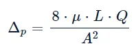
In non-ideal fluid dynamics, the Hagen–Poiseuille equation, also known as the Hagen–Poiseuille law, Poiseuille's law, or Poiseuille's equation, is a physical law that gives the pressure drop in an incompressible and Newtonian fluid in laminar flow through a long cylindrical pipe of constant cross section.
The assumptions of the equation are that the fluid is incompressible and Newtonian; the flow is laminar through a pipe of constant circular cross-section that is substantially longer than its diameter, and there is no acceleration of the fluid in the pipe. For velocities and pipe diameters above a threshold value, the actual fluid flow is not laminar but turbulent, leading to larger pressure drops than calculated using the Hagen-Poiseuille equation.
In standard fluid kinetics notation
where,
Δp">ΔpΔ� is the pressure difference between the two ends,
L is the length of pipe,
μ is the dynamic viscosity,
Q is the vloumetric flow rate.
R is the pipe radius.
A is the cross-section of the pipe
The equation does not hold close to the pipe entrance.
This is a schematic representation of pipe flow. This is what the fluid profile looks like.
The layer in which shear viscous forces are significant is called the boundary layer. This boundary layer is a hypothetical concept. It divides the flow in the pipe into two areas:
- Boundary layer region: Region in which viscous effects and velocity changes are significant.
Region of irrotational (core) flow: Region in which viscous effects and velocity changes are negligible, also known as the inviscid core. - When the fluid is just entering the pipe, the thickness of the boundary layer gradually increases from zero in the direction of the fluid flow and finally reaches the center of the pipe and fills the entire pipe. This area from the pipe entrance to the point where the boundary layer covers the entire pipe is called the hydrodynamic entrance area, and the length of the pipe in this area is called the hydrodynamic entrance length. In this region the velocity profile develops and therefore the flow is called a hydrodynamically developing flow. After this region the velocity profile fully develops and continues unchanged. This region is called the hydrodynamically fully developed region.
Assume the following:
- The distance the fluid must travel to fully develop is given by the inlet length formula.
- The given Reynolds number is 2100. This means that the flow is laminar.
- The input length formula for Laminar is therefore given as follows:L/d=0.06.Re
- where L is the effective length; d is the pipe diameter and Re is the Reynolds number.
- Assuming a pipe diameter of 10 mm; by substituting the values, we get L = 1.2m;
Steps to follow
- First, the geometry is created in the Dict mesh block file, this is done by creating the file using Matlab code.
- The mesh is generated on demand.
Velocity and pressure bc are applied - The controlDict file is modified for the simulation run time and time step;
- After specifying the geometry, the simulation can be started by calling the command "icoFoam" in the terminal.
- The 'paraFoam' command helps open paraView
- The shear stress diagram is obtained by post-processing the velocity results obtained from OpenFOAM.
Matlab code;
%creating blockMeshdict file
clear all
close all
clc

% The Reynolds number
Re = 2100
% The Diameter of pipe
D = 0.004
% The Entry length of pipe
L =0.06*Re*D
% The total length of pipe
L_p = L+0.7
% Radius of pipe
r = D/2
% Angle of wedge (less than 5)
theta = 4
% Dynamic viscosity
mu = 0.89e-3
% Density
rho = 997

% Hagen poiseuille flow equations
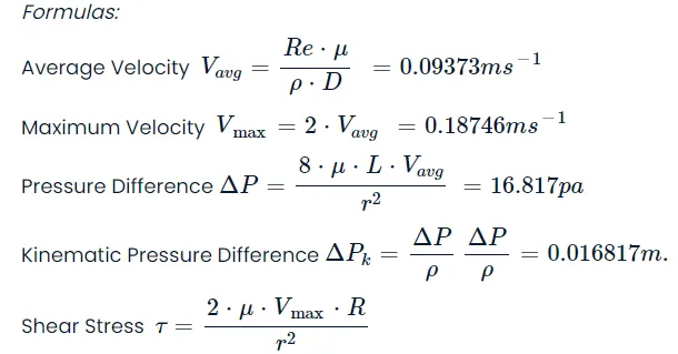
v_avg = (Re*mu)/(rho*D)
v_max = 2*(v_avg)
del_p = (8*mu*L_p*v_avg)/(r^2)
kinematic_p = del_p/rho

% calculating shear stress
R = linspace(0,(D/2),1000)

for i = 1:length(R)
    tau(i) = 2*mu*v_max*(abs(R(i)))/r^2
end

plot(R,tau)
xlabel("Radius")
ylabel("Shear stress")
grid on
legend ("Shear stress")


header1='/*----------------------------------*- C++ -*------------------------------------*'
header2='  =========                           |                                             '
header3='         /  F ield                | OpenFOAM: The Open Source CFD Toolbox       '
header4='        /   O peration            | Website:  https://openfoam.org              '
header5='       /    A nd                  | Version:  10                                '
header6='      /     M anipulation         |                                             '
header7='*----------------------------------------------------------------------------------*/'

f1 = fopen('blockMeshDict','w')
fprintf(f1, '%sn', header1)
fprintf(f1, '%sn', header2)
fprintf(f1, '%sn', header3)
fprintf(f1, '%sn', header4)
fprintf(f1, '%sn', header5)
fprintf(f1, '%sn', header6)
fprintf(f1, '%sn', header7)

fprintf(f1, 'FoamFilen{n')
fprintf(f1, '%12s t 2.0;n','version')
fprintf(f1, '%12s t ascii;n','format')
fprintf(f1, '%12s t dictionary;n','class')
fprintf(f1, '%12s t blockMeshDict;n','object')
fprintf(f1, '}n')
header8='// * * * * * * * * * * * * * * * * * * * * * * * * * * * * * * * * * * * * * //'
fprintf(f1, '%snn',header8)


fprintf(f1, 'convertToMeters 1;nn')

fprintf(f1, 'verticesn')
fprintf(f1, '(n')
fprintf(f1, 't (%d  %d %d)n',0,0,0)
fprintf(f1, 't (%d  %d %d)n',0,r*cosd(theta/2),r*sind(theta/2))
fprintf(f1, 't (%d  %d %d)n',0,r*cosd(theta/2),-r*sind(theta/2))
fprintf(f1, 't (%d  %d %d)n',L_p,0,0)
fprintf(f1, 't (%d  %d %d)n',L_p,r*cosd(theta/2),r*sind(theta/2))
fprintf(f1, 't (%d  %d %d)n',L_p,r*cosd(theta/2),-r*sind(theta/2))
fprintf(f1, ');nn')


fprintf(f1, 'blocksn')
fprintf(f1, '(n')
fprintf(f1, 't hex (0 3 5 2 0 3 4 1) (%d %d %d)',300,30,1)
fprintf(f1, ' SimpleGrading (1 0.1 1)nn')
fprintf(f1, ');nn')

fprintf(f1, 'edgesn')
fprintf(f1, '(n')
fprintf(f1, 't arc %d %d (%d %d %d)n',1,2,0,r,0)
fprintf(f1, 't arc %d %d (%d %d %d)n',4,5,L_p,r,0)
fprintf(f1, ');nn')

fprintf(f1, 'boundaryn')
fprintf(f1, '(n')
fprintf(f1, 't inlet n')
fprintf(f1, 't {n')
fprintf(f1, 'tt type patch;n')
fprintf(f1, 'tt facesn')
fprintf(f1, 'tt (n')
fprintf(f1, 'ttt (0 1 2 0)n')
fprintf(f1, 'tt );n')
fprintf(f1, 't }n')


fprintf(f1, 't outletn')
fprintf(f1, 't {n')
fprintf(f1, 'tt type patch;n')
fprintf(f1, 'tt facesn')
fprintf(f1, 'tt (n')
fprintf(f1, 'ttt (3 5 4 3)n')
fprintf(f1, 'tt );n')
fprintf(f1, 't }n')


fprintf(f1, 't topn')
fprintf(f1, 't {n')
fprintf(f1, 'tt type wall;n')
fprintf(f1, 'tt facesn')
fprintf(f1, 'tt (n')
fprintf(f1, 'ttt (1 4 5 2)n')
fprintf(f1, 'tt );n')
fprintf(f1, 't }n')

fprintf(f1, 't frontn')
fprintf(f1, 't {n')
fprintf(f1, 'tt type wedge;n')
fprintf(f1, 'tt facesn')
fprintf(f1, 'tt (n')
fprintf(f1, 'ttt (0 3 4 1)n')
fprintf(f1, 'tt );n')
fprintf(f1, 't }n')

fprintf(f1, 't backn')
fprintf(f1, 't {n')
fprintf(f1, 'tt type wedge;n')
fprintf(f1, 'tt facesn')
fprintf(f1, 'tt (n')
fprintf(f1, 'ttt (0 2 5 3)n')
fprintf(f1, 'tt );n')
fprintf(f1, 't }n')

fprintf(f1, 't axisn')
fprintf(f1, 't {n')
fprintf(f1, 'tt type empty;n')
fprintf(f1, 'tt facesn')
fprintf(f1, 'tt (n')
fprintf(f1, 'ttt (0 3 3 0)n')
fprintf(f1, 'tt );n')
fprintf(f1, 't }n')
fprintf(f1, '); nn')

fprintf(f1, 'mergePatchPairsn')
fprintf(f1, '(n')
fprintf(f1, ');n')

header9='// * * * * * * * * * * * * * * * * * * * * * * * * * * * * * * * * * * * * * //'
fprintf(f1, '%sn',header9)

fclose(f1)
The blockMeshDict file for a wedge with symmetrical boundary conditions is as follows:
BlockMeshDict file For
/*--------------------------------*- C++ -*----------------------------------*
  =========                 |
        /  F ield         | OpenFOAM: The Open Source CFD Toolbox
       /   O peration     | Website:  https://openfoam.org
      /    A nd           | Version:  10
     /     M anipulation  |
*---------------------------------------------------------------------------*/
FoamFile
{
    format      ascii;
    class       dictionary;
    object      blockMeshDict;
}
// * * * * * * * * * * * * * * * * * * * * * * * * * * * * * * * * * * * * * //

convertToMeters 1;

vertices
(
    (0.000000 0.000000 0.000000)
    (0.000000 0.009962 -0.000872)
    (0.000000  0.009962 0.000872)
    (2.5200000 0.000000 0.000000)
    (2.520000 0.009962 -0.000872)
    (2.520000 0.009962 0.000872)

);

blocks
(
    hex (0 1 2 0 3 4 5 3) (50 1 200) simpleGrading (0.5 1 1)
);

edges
(
            arc 1 2 (0.000000 0.010000 0.000000)
            arc 4 5 (2.520000 0.010000 0.000000)
);

boundary
(
    inlet
    {
        type patch;
        faces
        (
            (0 1 2 0)
        );
    }
    outlet
    {
        type patch;
        faces
        (
            (3 4 5 3)

        );
    }
    front
    {
        type symmetry;
        faces
        (
            (0 3 5 2)
        );
    }

    back
    {
        type symmetry;
        faces
        (
            (0 1 4 3)
        );
    }


    pipe
    {
        type wall;
        faces
        (
            (1 4 5 2)
        );
    }
    axis
    {
        type empty;
        faces
        (
            (0 3 3 0)
        );
    }


);

mergePatchPairs
(
);

// **************************************************************** //
BlockMeshDict file For
/*--------------------------------*- C++ -*----------------------------------*
  =========                 |
        /  F ield         | OpenFOAM: The Open Source CFD Toolbox
       /   O peration     | Website:  https://openfoam.org
      /    A nd           | Version:  10
     /     M anipulation  |
*---------------------------------------------------------------------------*/
FoamFile
{
    format      ascii;
    class       dictionary;
    object      blockMeshDict;
}
// * * * * * * * * * * * * * * * * * * * * * * * * * * * * * * * * * * * * * //

convertToMeters 1;

vertices
(
    (0.000000 0.000000 0.000000)
    (0.000000 0.009763 -0.002164)
    (0.000000  0.009763 0.002164)
    (2.5200000 0.000000 0.000000)
    (2.520000 0.009763 -0.002164)
    (2.520000 0.009763 0.002164)

);

blocks
(
    hex (0 1 2 0 3 4 5 3) (50 1 200) simpleGrading (0.5 1 1)
);

edges
(
            arc 1 2 (0.000000 0.010000 0.000000)
            arc 4 5 (2.520000 0.010000 0.000000)
);

boundary
(
    inlet
    {
        type patch;
        faces
        (
            (0 1 2 0)
        );
    }
    outlet
    {
        type patch;
        faces
        (
            (3 4 5 3)

        );
    }
    front
    {
        type symmetry;
        faces
        (
            (0 3 5 2)
        );
    }

    back
    {
        type symmetry;
        faces
        (
            (0 1 4 3)
        );
    }


    pipe
    {
        type wall;
        faces
        (
            (1 4 5 2)
        );
    }
    axis
    {
        type empty;
        faces
        (
            (0 3 3 0)
        );
    }


);

mergePatchPairs
(
);

// **************************************************************** //
BlockMeshDict file For
/*--------------------------------*- C++ -*----------------------------------*
  =========                 |
        /  F ield         | OpenFOAM: The Open Source CFD Toolbox
       /   O peration     | Website:  https://openfoam.org
      /    A nd           | Version:  10
     /     M anipulation  |
*---------------------------------------------------------------------------*/
FoamFile
{
    format      ascii;
    class       dictionary;
    object      blockMeshDict;
}
// * * * * * * * * * * * * * * * * * * * * * * * * * * * * * * * * * * * * * //

convertToMeters 1;

vertices
(
    (0.000000 0.000000 0.000000)
    (0.000000 0.009239 -0.003827)
    (0.000000  0.009239 0.003827)
    (2.5200000 0.000000 0.000000)
    (2.520000 0.009239 -0.003827)
    (2.520000 0.009239 0.003827)

);

blocks
(
    hex (0 1 2 0 3 4 5 3) (50 1 200) simpleGrading (0.5 1 1)
);

edges
(
            arc 1 2 (0.000000 0.010000 0.000000)
            arc 4 5 (2.520000 0.010000 0.000000)
);

boundary
(
    inlet
    {
        type patch;
        faces
        (
            (0 1 2 0)
        );
    }
    outlet
    {
        type patch;
        faces
        (
            (3 4 5 3)

        );
    }
    front
    {
        type symmetry;
        faces
        (
            (0 3 5 2)
        );
    }

    back
    {
        type symmetry;
        faces
        (
            (0 1 4 3)
        );
    }


    pipe
    {
        type wall;
        faces
        (
            (1 4 5 2)
        );
    }
    axis
    {
        type empty;
        faces
        (
            (0 3 3 0)
        );
    }


);

mergePatchPairs
(
);

// **************************************************************** //
The data relating to simulation time duration etc is updated in controlDict file as shown below:
controlDict file
/*--------------------------------*- C++ -*----------------------------------*
  =========                 |
        /  F ield         | OpenFOAM: The Open Source CFD Toolbox
       /   O peration     | Website:  https://openfoam.org
      /    A nd           | Version:  10
     /     M anipulation  |
*---------------------------------------------------------------------------*/
FoamFile
{
    format      ascii;
    class       dictionary;
    location    "system";
    object      controlDict;
}
// * * * * * * * * * * * * * * * * * * * * * * * * * * * * * * * * * * * * * //

application     icoFoam;

startFrom       startTime;

startTime       0;

stopAt          endTime;

endTime         10;

deltaT          0.001;

writeControl    timeStep;

writeInterval   20;

purgeWrite      0;

writeFormat     ascii;

writePrecision  6;

writeCompression off;

timeFormat      general;

timePrecision   6;

runTimeModifiable true;


// *************************************************************************
The boundary conditions can be given as follows. The velocity boundary condition was inserted in the problem discuss below.
velocity file
/*--------------------------------*- C++ -*----------------------------------*
  =========                 |
        /  F ield         | OpenFOAM: The Open Source CFD Toolbox
       /   O peration     | Website:  https://openfoam.org
      /    A nd           | Version:  10
     /     M anipulation  |
*---------------------------------------------------------------------------*/
FoamFile
{
    format      ascii;
    class       volVectorField;
    object      U;
}
// * * * * * * * * * * * * * * * * * * * * * * * * * * * * * * * * * * * * * //
dimensions      [0 1 -1 0 0 0 0];

internalField   uniform (0 0 0);

boundaryField
{
    inlet
    {
        type            fixedValue;
        value           uniform (0.0937312 0 0);
    }

    outlet
    {
        type            zeroGradient;
    }

    pipe
    {
        type            noSlip;
    }
    axis
     {
        type             empty;

      }
    front
     {
      type              symmetry;
       }


      back
     {
      type                symmetry;
     }


}

//**********************************//
The boundary conditions can be given as follows. The pressure drop boundary condition was inserted in the problem discussed below.
pressure file
/*--------------------------------*- C++ -*----------------------------------*
  =========                 |
        /  F ield         | OpenFOAM: The Open Source CFD Toolbox
       /   O peration     | Website:  https://openfoam.org
      /    A nd           | Version:  10
     /     M anipulation  |
*---------------------------------------------------------------------------*/
FoamFile
{
    format      ascii;
    class       volScalarField;
    object      p;
}
// * * * * * * * * * * * * * * * * * * * * * * * * * * * * * * * * * * * * * //

dimensions      [0 2 -2 0 0 0 0];

internalField   uniform 0;

boundaryField
{
    axis
    {
        type            empty;
    }

    pipe
    {
        type            zeroGradient;
    }

    inlet
    {
        type            zeroGradient;
    }

    outlet
    {
        type            fixedValue;
        value           uniform 0.0168682;
    }

    front
     {

     type                 wedge;

     }

     back
    {
     type                 wedge;
    }


}

// ************************************************************************* //
The data related to kinematic viscosity is updated in physicalProperties file.
/*--------------------------------*- C++ -*----------------------------------*
  =========                 |
        /  F ield         | OpenFOAM: The Open Source CFD Toolbox
       /   O peration     | Website:  https://openfoam.org
      /    A nd           | Version:  10
     /     M anipulation  |
*---------------------------------------------------------------------------*/
FoamFile
{
    format      ascii;
    class       dictionary;
    location    "constant";
    object      transportProperties;
}
// * * * * * * * * * * * * * * * * * * * * * * * * * * * * * * * * * * * * * //

nu              [0 2 -1 0 0 0 0] 8.927e-07;


// ************************************************************************* //
After checking the network, we get the following confirmation. At this stage, we can use ParaView and enter the paraFoam command to check whether our mesh meets the requirements or not.
With the mesh deployed we are now ready to run the simulation. The simulation we chose was icoFoam. So just type "icoFoam" and the simulation will start.
Output:
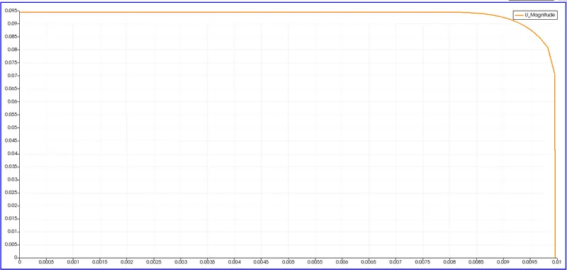
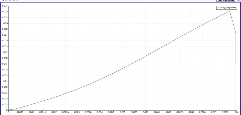
Results for a 10 degree wedge angle with symmetrical boundary conditions:
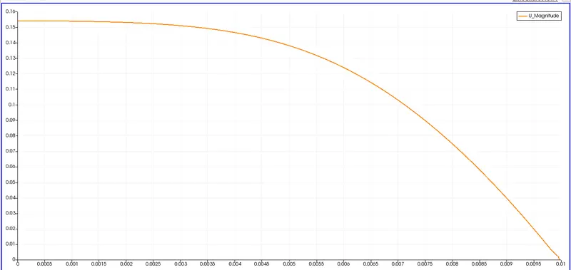
The velocity plots
At a distance of 0.001 from the inlet
At a distance of 0.5 from the inlet
At a distance of 1.15 from the inlet
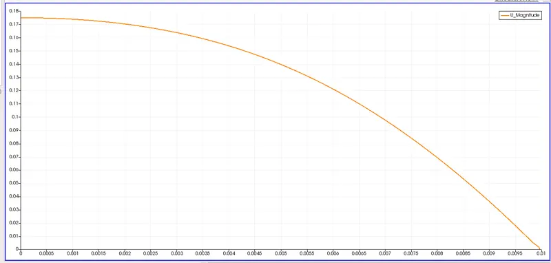
At the outlet
Shear stress in the almost fully developed regions is as follows:
Results for an angle of 25 degrees of a wedge with symmetrical boundary conditions:
The velocity plots
At a distance of 0.001 from the inlet
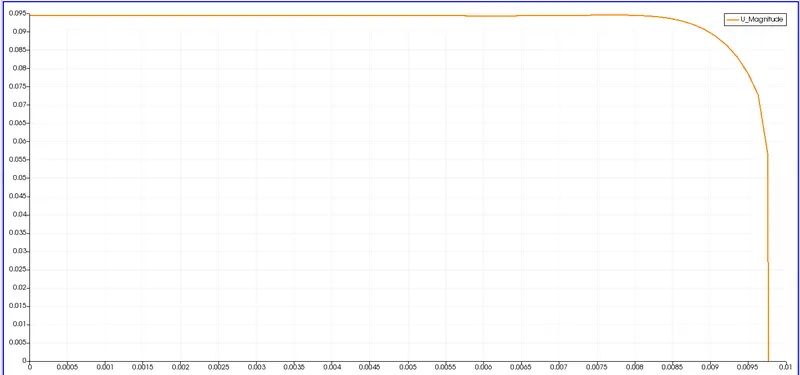
At a distance of 1.15 from the inlet
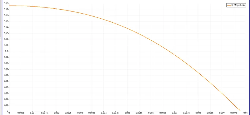
At the outlet
Shear stress in the almost fully developed regions is as follows:
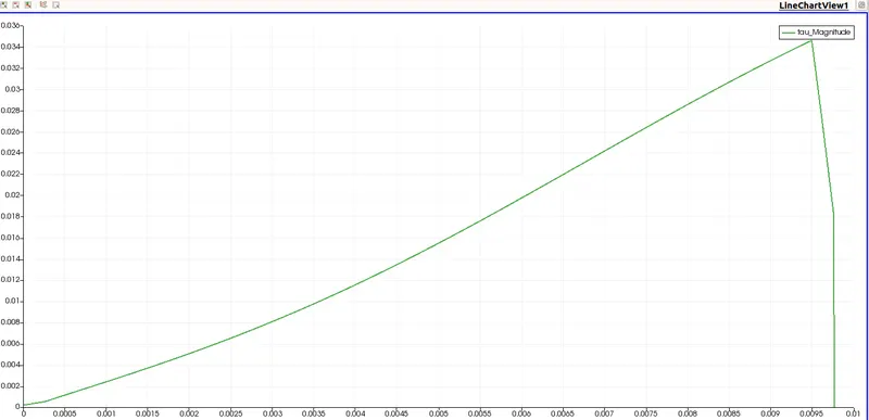
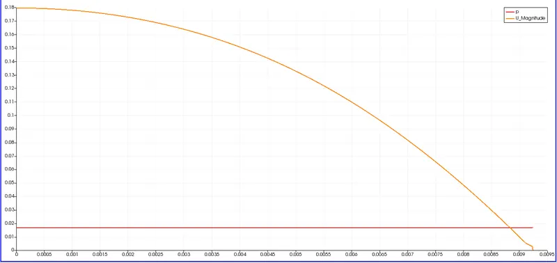
Results for an angle of 45 degrees of a wedge with symmetrical boundary conditions:
The velocity plots
At a distance of 0.001 from the inlet
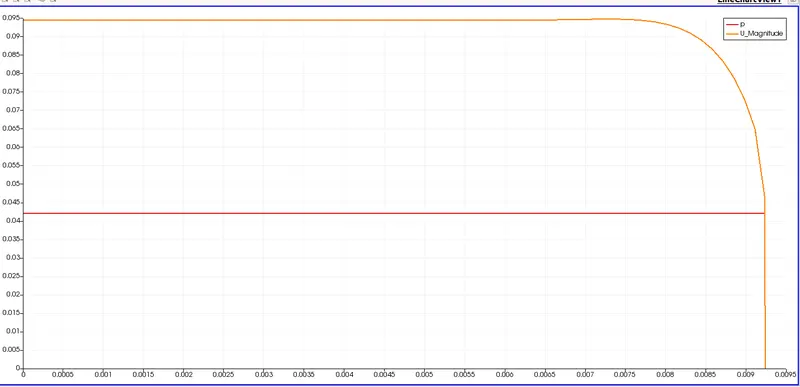
At a distance of 0.5 from the inlet:
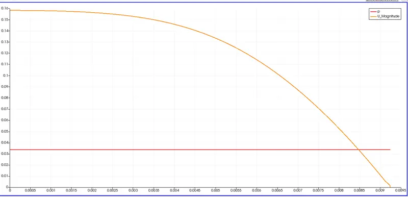
At a distance of 1.15 from the inlet
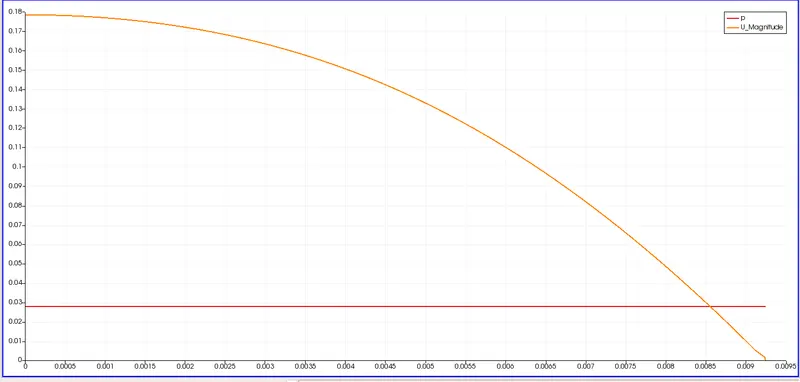
At the outlet
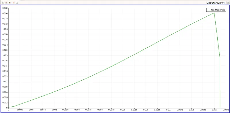
Shear stress in the almost fully developed regions is as follows:
Results
| Wedge angle in degrees | Max velocity(by equation) | Max velocity by simulation | Max shear stress |
| 10(Symmetry BC) | 0.1875 | 0.175861 | 0.034 |
| 25(Symmetry BC) | 0.1875 | 0.1770109 | 0.03451 |
| 45(Symmetry BC) | 0.1875 | 0.1796 | 0.03609 |
conclusions:
- Here we could see that as the wedge angle increases, the speed becomes more accurate to the actual value.
- We also observe that the symmetric BC is more accurate in terms of speed, where it is very close to the true value. This means that its accuracy is high.
- As observed, we could say that the symmetric BC takes more time to calculate or run the simulation because of its fine coupling.
- We could also observe that at the distance of 1.15 and 2.52 the velocity plots seem to be the same, which means that the distance of 1.15 is closer to the distance of the fully developed region.
- Due to the no-slip boundary conditions, the velocity is reduced to zero at the edge near the pipe walls in all cases.
- Also, the maximum shear stress is found in the walls of the pipe itself. and immediately drops to zero on Wednesday.
- As the wedge angle increases, the courant number increases, which can be explained by the increase in the size of the mesh elements, since the number of elements remains the same in the analysis. The courant number is directly proportional to the size of the element