Calculating Hill Climbing Power of a TATA Ultra Truck, flyover

Aims:

1. To find the ratio of hill-climbing power required by fully loaded tata ultra truck to the half-loaded one.
2. To find the minimum length of the flyover, considering the minimum height at the summit should be 5 meters.
3. To prepare a new drive cycle excel file for the Driver Glider model by Simulink and also include a hill-climbing angle. Revise the model according to the new data and comment on the results.
4. To model the WOT (Wide Open Throttle) response of GM EV1 car. To compare it with the official figures of the performance of a real vehicle and to prepare a table showing variation in acceleration time with a 5% change in vehicle parameters.

Theory:

Part 1: To find hill-climbing ratio of TATA Ultra truck, with full and half loading.

TATA T.12 Ultra Day Truck was considered for calculations. The specifications of the vehicle is as shown below [1].

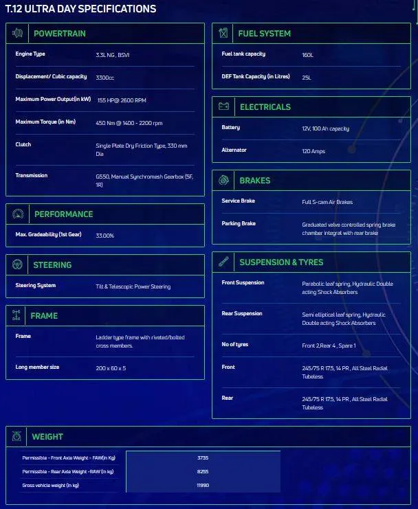
Parameters of vehicles for calculations:

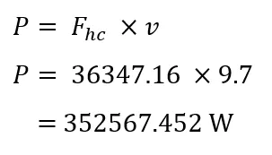
1) Calculations for fully loaded vehicle:

Vehicle kerb weight (kg): 3735

Vehicle payload weight (kg): 8255

Gross Vehicle weight (kg): Vehicle kerb weight + Vehicle payload weight = 11990

Speed (v) = 35km/hr = 9.7 m/s

Gradeability (ϴ) = 33% = 18.26° [2]

As we know, the hill climbing force (F_hc) is given by:

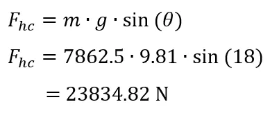
2) Calculations for half loaded vehicle:

Vehicle kerb weight (kg): 3735

Vehicle payload weight (kg): 8255/2 = 4127.5

Gross Vehicle weight (kg): Vehicle kerb weight + Vehicle payload weight = 7862.5

Speed (v) = 35km/hr = 9.7 m/s

Gradeability (ϴ) = 33% = 18.26° [2]

As we know, the hill climbing force (F_hc) is given by:

Now total power required (P) is given by:

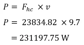
Now, the ratio of fully loaded VS half loaded

Therefore, the ratio is 1.5

Part 2: To find the minimum length of the flyover, considering the minimum height at the summit should be 5.5 meters.

Here the given minimum summit height is 5.5 m

Considering the gradeability of the vehicle as 18°

Therefore, the minimum length of the flyover can be calculated by:

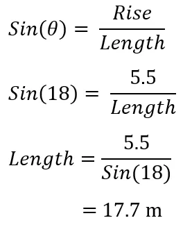
Therefore, the minimum length of the flyover should be 17.7 m.

Part 3: To prepare a new drive cycle excel file for the Driver Glider model by Simulink including hill climb angle and to comment on the results.

The drive cycle created for the Driver Glider model is as shown in the figure below, where the time ranged from 1 to 220 seconds and the velocity from 0 to 100 km/hr, however, the velocity was then converted to m/s for the model and the later values were used for the input in the model.

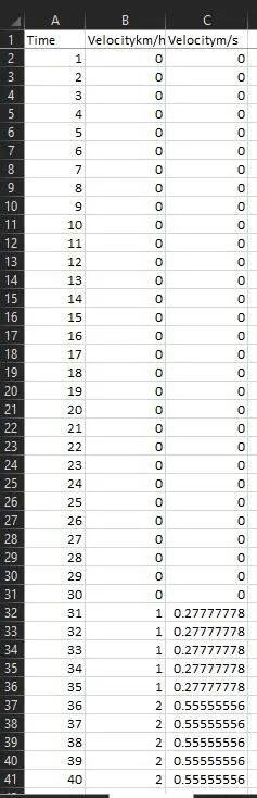
The google sheet (link) for these values is as given below.

https://docs.google.com/spreadsheets/d/1JmVbe0K1hb7W4Hcax7nkTBHcFUr91FQFGWeniTBLUT8/edit?usp=sharing

The values of the drive cycle were then exported into Matlab workspace by selecting only the Time and Velocity m/s values, converting them into numerical values from the top “Output Type” selection.

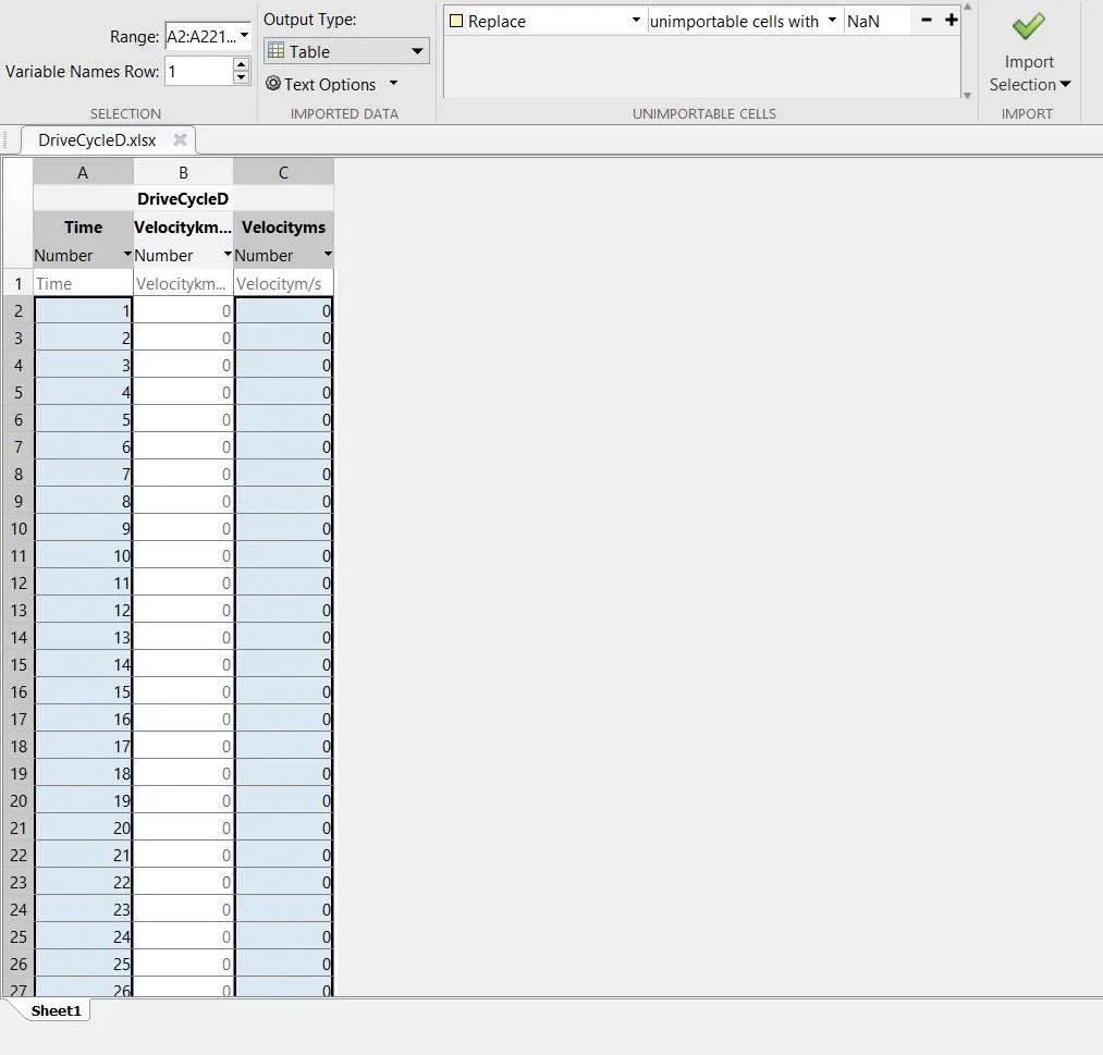
The values were then inserted into Simulink model using the “from workspace” block of Simulink. The Simulink model for driver glider model is as shown below.

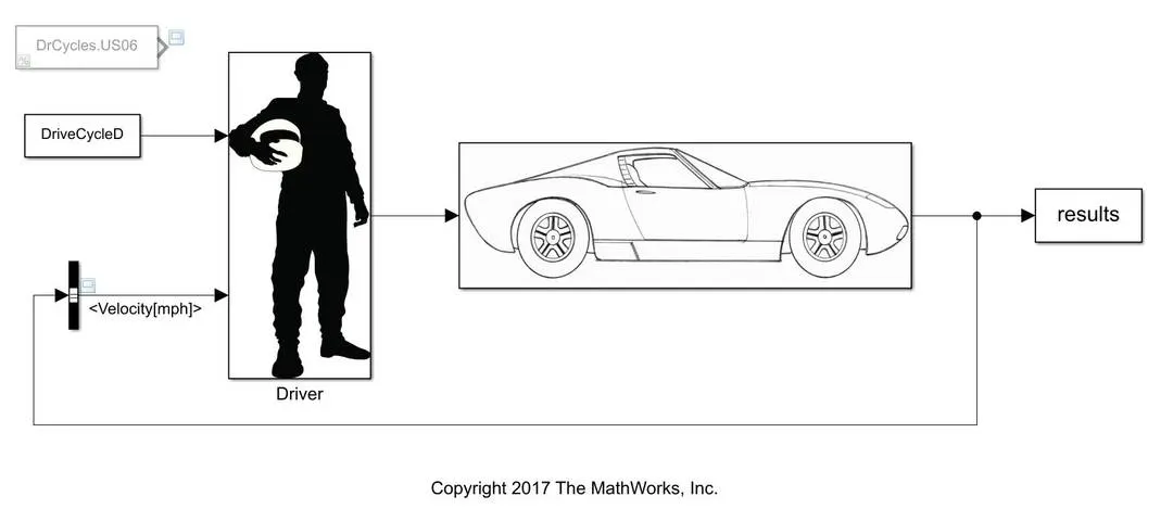
Here we can see the “DriveCycleD” block of the drive cycle inserted for the modified simulation of the model. Thereafter the inclination grade angle was changed from 0 to 18 of the car to observe the changes in the output.

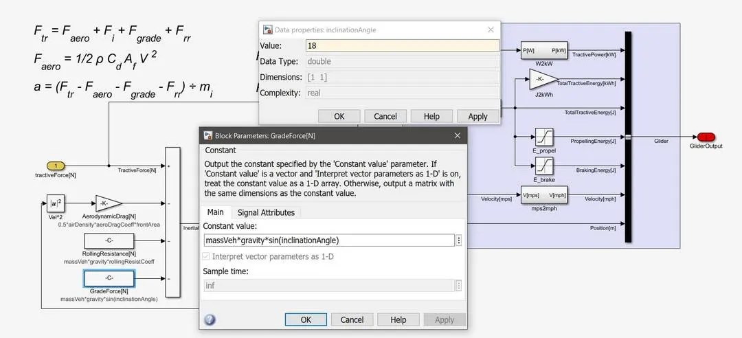
For this some alterations were done into the model where we can observe both the outputs at the same time, which can be seen in the figure below.

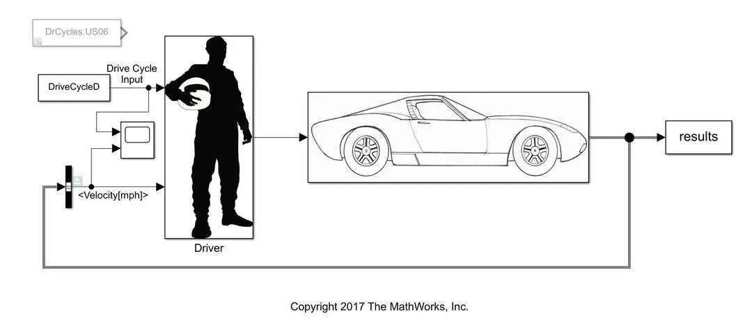
Here a scope was inserted between the input values of the drive cycle and the output of the Velocity of the vehicle. The output of the simulation can be seen below.

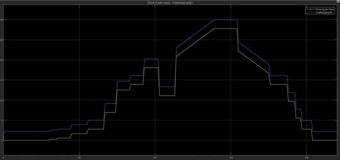
As seen above the green plot is the input values of the drive cycle and the blue plot is the output values of the simulation with the hill climbing inclination angle given to the vehicle.

It is observed that the velocity has increased compared to the input values, because of the inclination angle.

Part 4: To model the WOT (Wide Open Throttle) response of GM EV1 car and to compare the response of the car with original parameters and 5% varied parameters.

The governing equation of acceleration of the vehicle is as below.

The parameters assumed for the vehicle are as below:

m: mass of the vehicle(kg) = 1000

r: tire radius(m) = 0.30

G: gear ratio = 11

v: velocity(m/s) = 19.8

Cd = coefficient of drag = 0.19

u_rr = rolling resistance = 0.0048

T = Max torque(Nm) = 140

a = frontal area(m²) = 1.8

n_g = gear efficiency = 0.95

dv/dt = acceleration of vehicle.

Part A: Calculations with the original parameters of the vehicle.

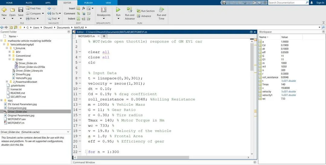
The Matlab code of the calculations is as shown below

% WOT(wide open throttle) response of GM EV1 car

clear all
close all
clc

% Input Data
t = linspace(0,30,301);
velocity = zeros(1,301);
dt = 0.10;
Cd = 0.19; % drag coefficient
roll_resistance = 0.0048; %Rolling Resistance
m = 1000; % Vehicle Mass
G = 11; % Gear Ratio
r = 0.30; % Tire radius
Tmax = 140; % Motor Torque in Nm
wc = 733; % 
v = 19.8; % Velocity of the vehicle
a = 1.8; % Frontal Area
eff = 0.95; % Efficiency of gear

% Calculating WOT of GM EV1 with original parameters
for n = 1:300
    if velocity(n)<19.8
        velocity(n+1) = velocity(n)+dt*(3.08-(0.00137*(velocity(n)^2)));
    else if velocity(n)>19.8
            velocity(n+1) = velocity(n)+dt*((62.1/velocity(n))-0.046-(0.000137*(velocity(n)^2)));
        end
        if velocity(n)>36
            velocity(n+1)=velocity(n);
        end
    end
end

% Now plotting WOT of GM EV1 having original parameters
velocity = velocity*3.6; % converting m/s to km/hr
figure(1)
plot(t,velocity)
axis([0 35 0 150])
xlabel('Time (sec)')
ylabel('Velocity (km/hr)')
title('Wide Open Throttle of GM EV1 with original parameters')
legend('Original Parameters','Location','northwest')
grid on

The plot of the above calculation for the vehicle with original parameters is as shown below.

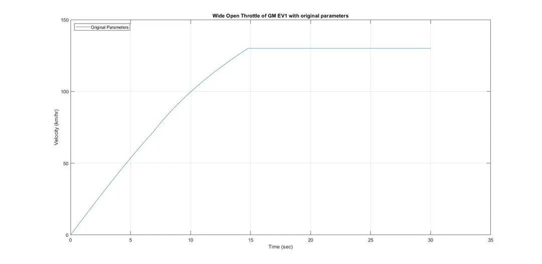
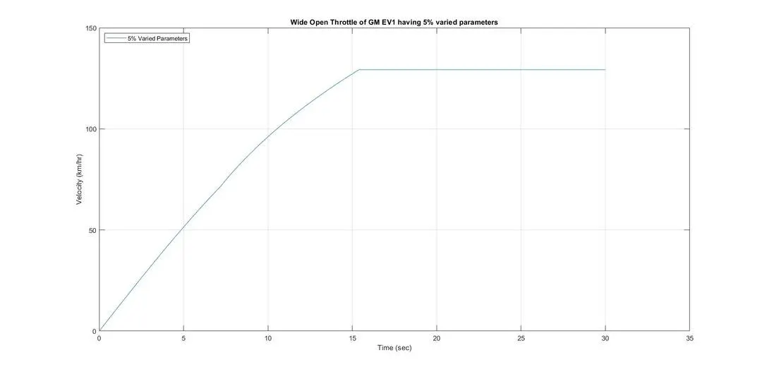
Part B: The Matlab code for the vehicle with 5% varied parameters where the mass of the vehicle was considered as 1050 kg and the frontal area as 1.9 m². Therefore, the calculations carried out are:

% Calculating WOT of GM EV1 varied by 5%
% Input data considered
m1 = 1050;
G1 = 11;
a = 1.9;
velocity1 = 0;

for n = 1:300
    if velocity1(n)<19.8
        velocity1(n+1) = velocity1(n)+dt*(2.95-(0.00137*(velocity1(n)^2)));
    else if velocity1(n)>19.8
            velocity1(n+1) = velocity1(n)+dt*((59.14/velocity1(n))-0.046-(0.000137*(velocity1(n)^2)));
        end
        if velocity1(n)>35.8
            velocity1(n+1)=velocity1(n);
        end
    end
end

% Now plotting WOT of GM EV1 having 5% varied parameters
velocity1 = velocity1*3.6; % converting m/s to km/hr
figure(2)
plot(t,velocity1)
axis([0 35 0 150])
xlabel('Time (sec)')
ylabel('Velocity (km/hr)')
title('Wide Open Throttle of GM EV1 having 5% varied parameters')
legend('5% Varied Parameters','Location','northwest')
grid on

The plot of the above calculation for the vehicle with 5% varied parameters is as shown below.

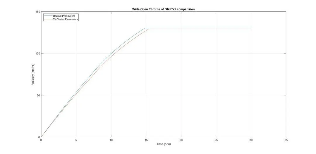
Now both the parameters were compared by plotting both the above graphs into one graph. For which the Matlab code is as shown below.

% Comparing both plots
figure(3)
plot(t,velocity)
hold on
plot(t,velocity1)
axis([0 35 0 150])
xlabel('Time (sec)')
ylabel('Velocity (km/hr)')
title('Wide Open Throttle of GM EV1 Comparision')
legend('Original Parameters','5% Varied Parameters','Location','northwest')
grid on

The result plot is as shown below.

The screenshot of the Matlab environment coding with results in Matlab is as shown below

Conclusions:

1. The ratio of the power required by TATA Ultra truck with fully loaded vehicle and half loaded vehicle is 1.5.
2. The minimum length of the flyover was calculated and it came out to be 17.7 meters.
3. The simulation of the Driver Glider model with a new Drive Cycle and added new inclination hill climbing angle was carried out successfully. It was observed that the velocity has increased compared to the input values, because of the inclination angle.
4. The calculations for the Wide Open Throttle for GM EV1 were done successfully with the aid of Matlab coding and the calculations with original vehicle parameters and with 5% varied parameters were done and were compared in a single plot. It was observed that the acceleration time was increased because of the 5% variation of the vehicle parameters.

References:

[1] https://light-trucks.tatamotors.com/light-trucks/icv-diesel-trucks/10-tonne-12-tonne-trucks/tata-t12-ultra-day-specifications.aspx

[2] https://www.calcunation.com/calculator/slope-percent-conversion.php