To calculate work done by a cutting tool, to model a governing equation and save it to external file and to analyse

Aims:

1. To find the work done by the cutting tool with the given data of distance travelled and force applied.
2. To make a model for the given equation and to save the output to an external file directed from the Simulink model.
3. To analyse the Simulink example ‘Mass-Spring-Damper in Simulink and Simscape’.

Objectives:

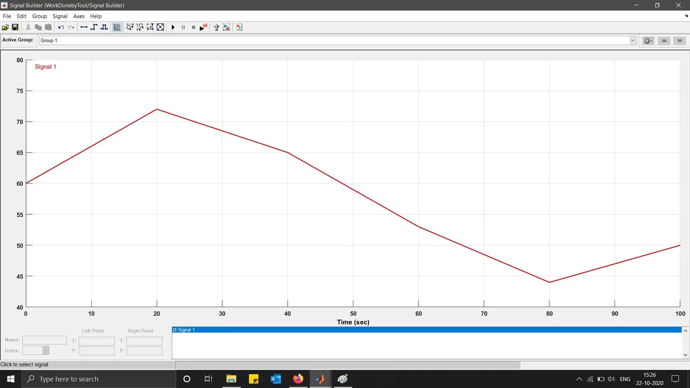
To determine the work done as the tool moves through a distance of 100 mm for the given set of data:

Distance (mm)	0	20	40	60	80	100
Force (kN)	60	72	65	53	44	50

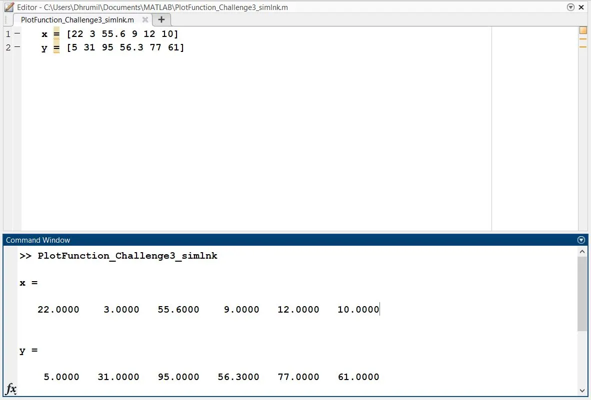
2. To make a Simulink model for a given equation and store the result using “To File” block in Simulink. The given variables for x and y are:

x = [22 3 55.6 9 12 10]

y = [5 31 95 56.3 77 61]

3. To find the Simulink model ‘Mass-Spring-Damper in Simulink and Simscape’ in Simulink help, to run and analyse the output and solve the following problems:

1. To derive the equation for the model.
2. Change the value of mass, damper, and spring for the Simscape model and plot the result. Change the value of Mass x0=2 in the Simulink model and plot the results.
3. Make the response from Simscape and Simulink as two separate displays

Theory:

Part 1: Determine work done by the tool

The Simulink model as shown below was made to calculate the work done by the tool.

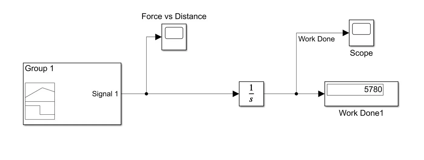
The signal builder was used to give the force and distance inputs via signals as seen below.

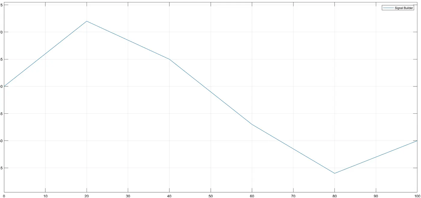
Which were then observed by the scope connected after the signal builder.

The input signal was then integrated using an integrator block and the output was received by the output scope and the answer displayed on the display block was 5780. The output scope plot is as shown below. The resulting nature of the plot is discussed in the results section at the end of the project.

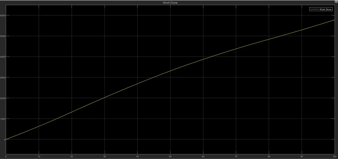
Note: Snipping tool was used to save the plot figure as the values of work done were not visible by saving through copying the plot to the clipboard and saving via paint.

Part 2: To create a Simulink model for a given equation and to save the result using "To File” block.

The Simulink model for the given equation is as shown below.

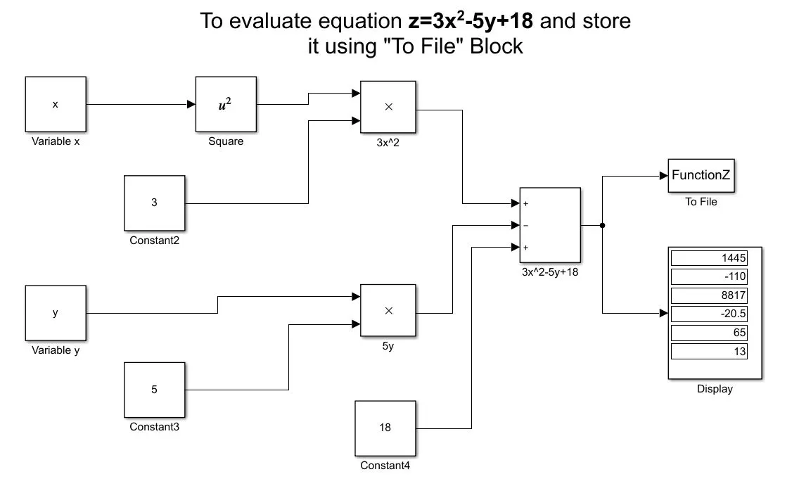
Here in the model common mathematical calculation blocks were used to form the equation. Variables x and y were stored in the Matlab workspace and thereafter were routed in the constant blocks in the initial stage of modelling.

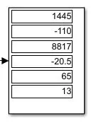
Thereafter the square, multiplication and addition/subtraction blocks were used to form the equation. Thereafter the answer was saved externally in the Matlab folder destination using “To File” block and a display was used to show the answers. The above visible answers were stored in the “FunctionZ.mat” file in the destination folder.

Answers in the display

The output of “FunctionZ.mat” file is as below.

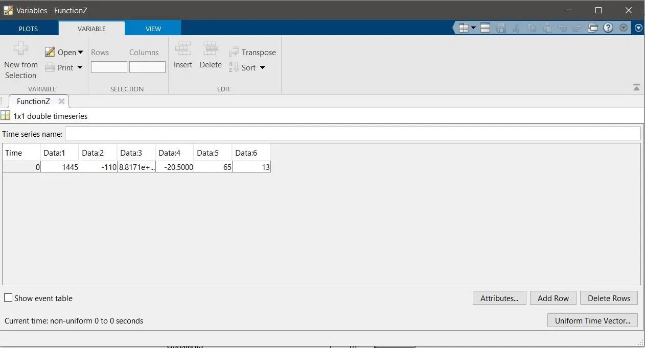
The saved file at the destination folder.

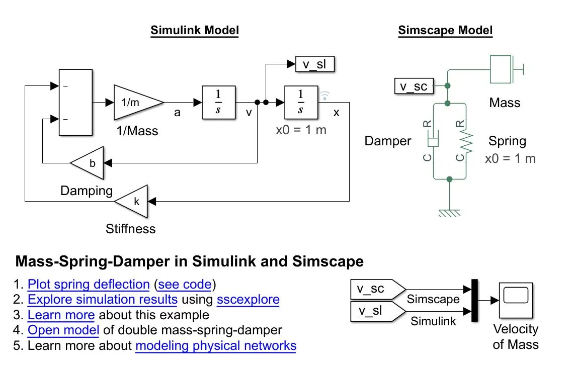
Part 3: To analyse the Simulink example ‘Mass-Spring-Damper in Simulink and Simscape’

The model of mass spring damper example of the Simulink is as shown below:

1) To derive the equation of the system:

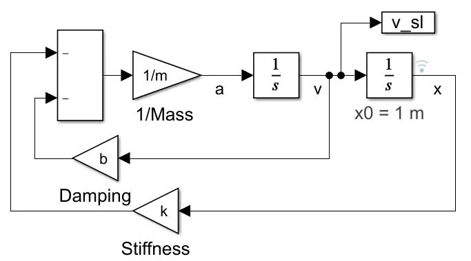
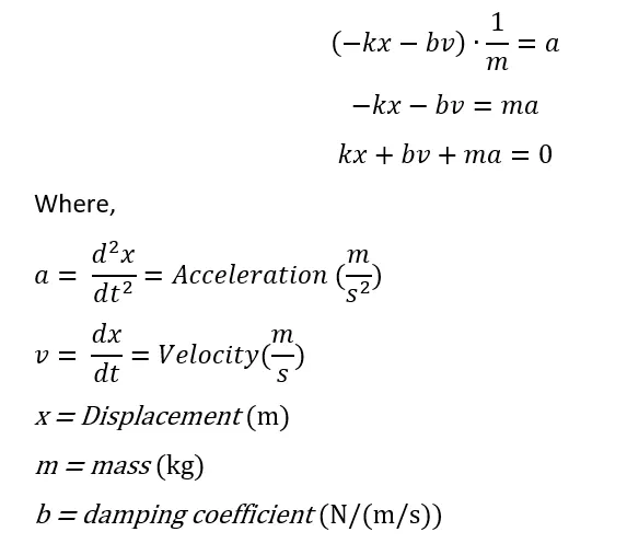
From the above figure

2) Change the value of mass, damper, and spring for the Simscape model.

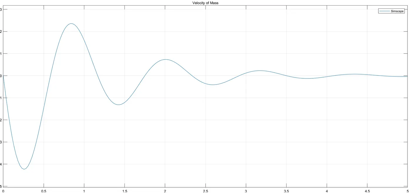
There were two cases where the mass, damper and spring coefficients were changed as listed below and then the graphs were plotted for the same.

	Spring (k) (N/m)	Mass (m) (kg)	Damper (b) (N/(m/s))
Case 1	300	10	20
Case 2	200	50	35

The plot for Case 1 is as below:

The plot for Case 2 is as shown below:

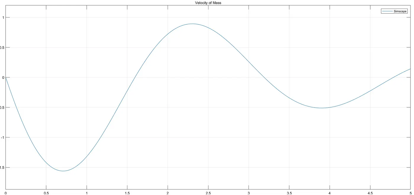
Thereafter the value of X0 was changed to 2 in the Simulink model where the graph observed is as shown below.

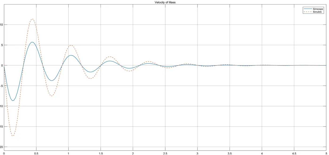
Over here, the models were compared with X0 = 2 and X0 =1, basically not changing the value of X0 in the Simscape model. In the plot above there was a large deflection was observed when the value of X0 is changed to 2. Where then got subsided along with the original wave. Here the intensity is more compared to mass X0=1.

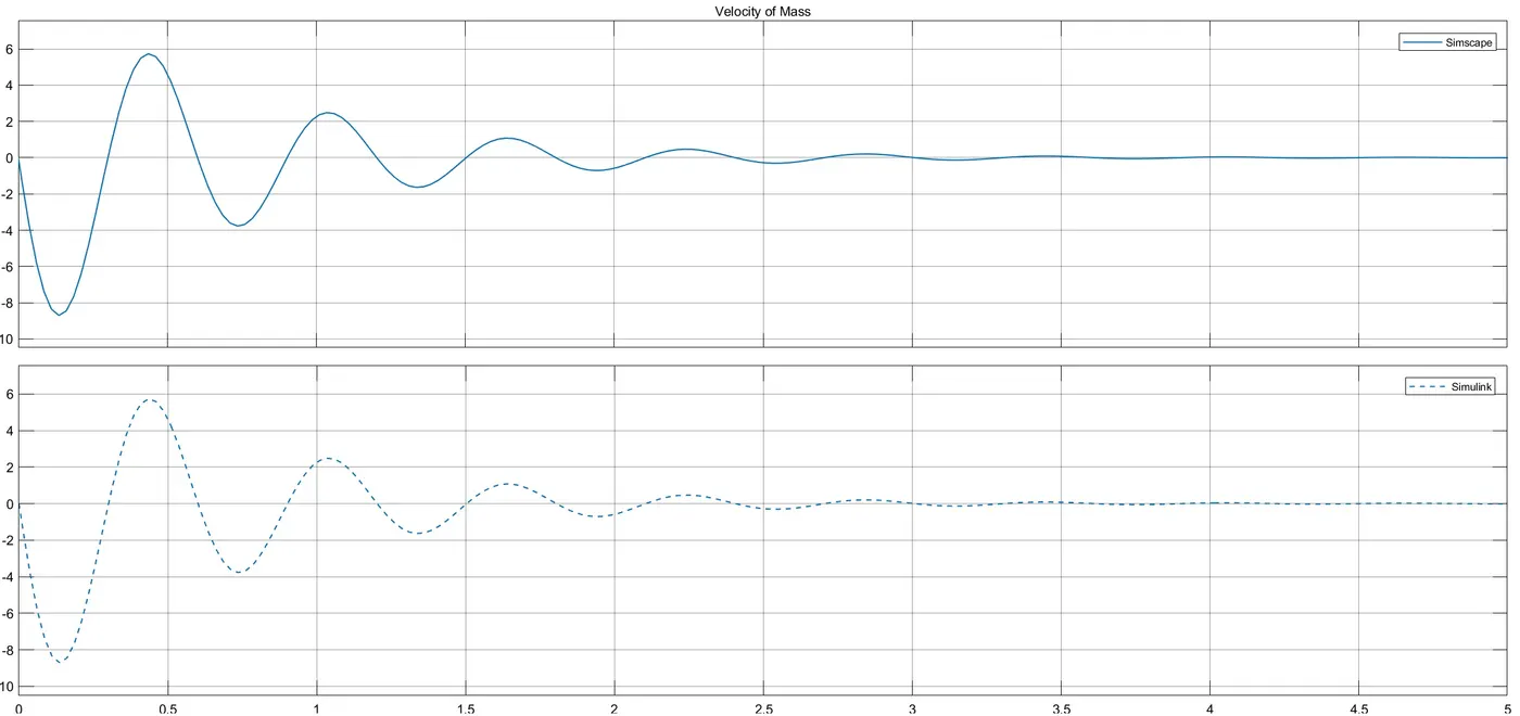
3) Make the response from Simscape and Simulink as two separate displays.

The output of both Simulink and Simscape models were observed separately by selecting the view option in the scope, where two windows were selected to view the plots separately as shown below. The graph plotted here is of the default data of spring, mass and damper given by MathWorks.

Results:

1. The work done by the tool was calculated which came to 5780, where in the graph we can see that as the time increased the work done increased exponentially.
2. The values for the governing equation were calculated and displayed which were then saved to a file “FunctionZ.mat” at the destination folder.
3. The equation for the spring, mass, damper system was derived, the plots for different values of spring, mass, damper were made successfully and the two plots for Simulink and Simscape models were separated successfully.