Simulation of Transient Motion of a Pendulum using Matlab

Aim:

To write a program in Matlab to solve second order ODE for a pendulum and to simulate an oscillating pendulum using the ODE calculations in Matlab.

Description:

In a pendulum, where a mass is hanging at the end of a string, where L is considered as the length of the string and “m” is considered to be the mass of the hanging object/sphere. The gravity “g” is considered in calculating the second order ODE equation, along with “b” which is the damping coefficient. As shown in the figure a sphere is hanging at the end of the string.

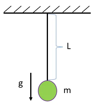
The equation of motion of a simple pendulum with damping is:

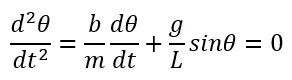
Here we can say the equation is a second order equation because of the d²θ has the square to it. The given parameters for a pendulum are:

g= gravity = 9.81 m/s²

L= length of the pendulum = 1 metre

b= damping coefficient = 0.05

m= mass = 1 kg

To calculate the ODE, we need to transform the given equation into a first order equation and further convert it into a function in Matlab and thereafter plotting it in Matlab software. Here the time span was determined along with angular displacement and angular velocity.

Once the angular momentum vs time plot is made, the simulation of the pendulum was done using the ODE calculations carried out. To simulate the pendulum, the length of the string was determined to plot the string, where the base of the pendulum was also determined from which the pendulum was hanged. Thereafter, the movements of the pendulum were defined by the calculations of ODE, which were used as input in the “for loop” to oscillate the pendulum from one point to another with in the given timeframe.

Theory:

% Solving second order ODE using Matlab

clear all
close all
clc

% Inputs
b = 0.05;
g = 9.81;
l = 1;
m = 1;

% Initial Condition
theta_0 = [0;3];

% Time Points
t_span = linspace(0,20,500);

% Solve ODE
[t,results] = ode45(@(t,theta) ode_func(t,theta,b,g,l,m), t_span, theta_0);

plot(t,results(:,1))
hold on
plot(t,results(:,2))
ylabel('Angular Momentum')
xlabel('Time')
title('Time vs Angular momentum')
legend('Displacement','Velocity','Location','northeast','orientation','horizontal')
ct=1;

% For Pendulum Animation

for i = 1:length(results(:,1))
    x0 = 0;
    y0 = 0;
    
    x1 = l*sind(results(i,1));
    y1 = -l*cosd(results(i,1));
    
    figure(2)
    plot([-1 1],[0 0], 'linewidth',4,'color','r');
    hold on
    
    line([x0 x1], [y0 y1], 'linewidth',2,'color','b');
    hold on
    
    plot(x1,y1, 'o', 'markers',40, 'markerfacecolor', 'g','markeredgecolor','m');
    
    grid on
    title('Pendulum Animation')
    axis([-1.3 1.3 -1.5 0.5])
    pause(0.01)
    
    hold off
    hold off
    
    M(ct) = getframe(gcf);
    
    ct = ct+1;
    
end

movie(M)
videofile = VideoWriter('Animation_of_Pendulum.avi','Uncompressed AVI');
open(videofile)
writeVideo(videofile,M)
close(videofile)

% Solving second order ODE using Matlab

clear all
close all
clc

Initially “% Solving second order ODE using Matlab” and “clear all” “close all” and “clc” were written to close all the running programs and clear the command window.

% Inputs
b = 0.05;
g = 9.81;
l = 1;
m = 1;

There after the inputs for the pendulum such as Damping factor “b”, Gravity “g”, length of the pendulum string “l” and mass “m” were inserted for the further calculations.

% Initial Condition
theta_0 = [0;3];

% Time Points
t_span = linspace(0,20,500);

Thereafter initial angular displacement and initial angular velocity were input into the program where initial angular displacement is 0 and initial angular velocity is 3 rad/sec. Then, the time span was defined between 0 to 20 seconds which was divided into 500 equal values, therefore the command “linspace” is used.

% Solve ODE
[t,results] = ode45(@(t,theta) ode_func(t,theta,b,g,l,m), t_span, theta_0);

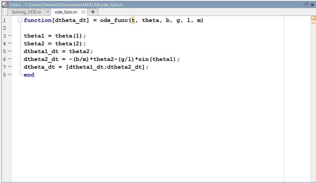
To solve the ODE function “ode_func” was defined in another program which was called out here for the calculations. ODE 45 is an inbuilt solver to solve first order functions in Matlab. The ODE45 uses integration to solve the first order differential equations that is defined in the function to give suitable result. The function programmed is as below.

function[dtheta_dt] = ode_func(t, theta, b, g, l, m)

theta1 = theta(1);
theta2 = theta(2);
dtheta1_dt = theta2;
dtheta2_dt = -(b/m)*theta2-(g/l)*sin(theta1);
dtheta_dt = [dtheta1_dt;dtheta2_dt];
end

Initially considering θ=θ₁,

Then,

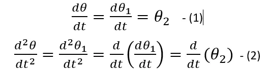
Here in the equation, replacing the values and creating two ODEs:

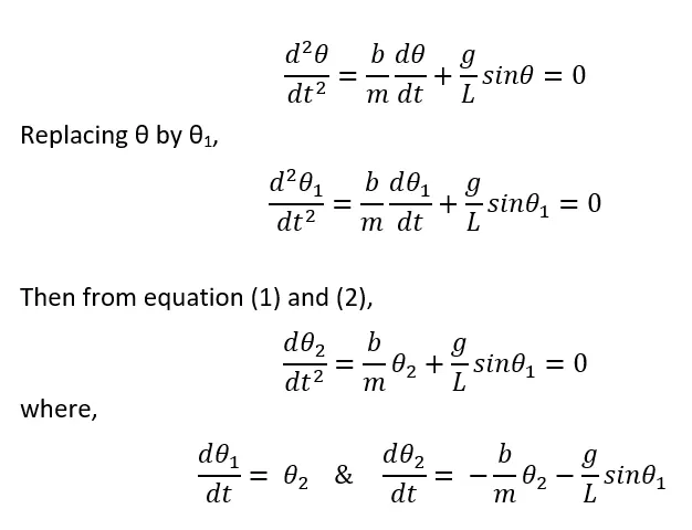
Therefore, in the program dtheta_dt = [dtheta1_dt;dtheta2_dt]; was written and the function loop was ended. Where “dthetha1_dt” was assigned to “theta2” and “dtheta2_dt” was assigned to “-(b/m)*theta2-(g/l)*sin(theta1)”.

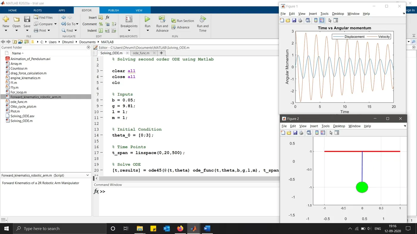
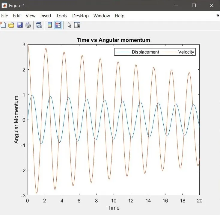
Therefore, by creating these two ODEs we get the values of displacement and velocity. As seen in the result plot of Time vs Angular Momentum the displacement starts from 0 and velocity starts from 3 which was our input, therefore the values were calculated by taking the inputs b, g, l ,m, theta, and time. Where theta and time were in range of values and others were a single value.

plot(t,results(:,1))
hold on
plot(t,results(:,2))
ylabel('Angular Momentum')
xlabel('Time')
title('Time vs Angular momentum')
legend('Displacement','Velocity','Location','northeast','orientation','horizontal')
ct=1;

For plotting our displacement and velocity the following “plot” command was used where “t” time versus “results(:,1)” that is displacement values and in the second plot command “results(:.2)” that is velocity values were plotted. Thereafter, the y-axis label and x-axis label were defined along with the legend and title for the plot. In the end the counter was set for the simulation purpose.

To simulate the oscillations of the pendulum the following program was written:

% For Pendulum Animation

for i = 1:length(results(:,1))
    x0 = 0;
    y0 = 0;
    
    x1 = l*sind(results(i,1));
    y1 = -l*cosd(results(i,1));
    
    figure(2)
    plot([-1 1],[0 0], 'linewidth',4,'color','r');
    hold on
    
    line([x0 x1], [y0 y1], 'linewidth',2,'color','b');
    hold on
    
    plot(x1,y1, 'o', 'markers',40, 'markerfacecolor', 'g','markeredgecolor','m');
    
    grid on
    title('Pendulum Animation')
    axis([-1.3 1.3 -1.5 0.5])
    pause(0.01)
    
    hold off
    hold off
    
    M(ct) = getframe(gcf);
    
    ct = ct+1;
    
end

Here to simulate the oscillating pendulum, “for loop” was used. As studied in the topic of “2R Robotic Arm” the simulation of Robotic arm was carried out. Learning from that the “for loop” was written. Where “i” was defined as “1:length(results(:,1))” that is 1 to the values of displacement as we want to simulate the displacement of the pendulum. Thereafter the x and y coordinates were defined to plot the pendulum. The base line from where the pendulum is hanging was defined by locating the x and y coordinates in the space and colouring it red by giving its thickness as 4. Then the string, at the end of which, the sphere is hanging was plotted by locating the x0, x1, y0 and y1 coordinates, colouring it blue and its thickness as 2. Lastly the sphere was located at the end of the string which was an “o” marker giving its dimension as 40 and colouring it green and colouring its edge as magenta. The technique for plotting a marker and customising were learnt from [1].

“Hold on” command were used twice in the “for loop” once before the string plotting and once before locating the sphere. As the string and the sphere are the moving parts of this simulation. There after the command to turn on the grid was given and the axis of the plot window were defined. Two “hold off” commands were used because there are two “hold on” commands used earlier, this was used as the simulating point will not stay at one point and will keep moving as required, because the axis remains the same and is not reset and clear the area. “getframe” command was used to get all the frames in one window to create a movie. The counter was set as original counter plus one so that there will not be a static graph with all the positions plotted at once. And hence the “for loop” was ended

movie(M)
videofile = VideoWriter('Animation_of_Pendulum.avi','Uncompressed AVI');
open(videofile)
writeVideo(videofile,M)
close(videofile)

The following commands were used to create the movie file. Where movie(M) was created where M was defined earlier in the “for loop”. The command “videofile” was used to create the avi file which was named Animation_of_ Pendulum.avi and the file was commanded to be uncompressed file. There after “open(videofile)” was used to start the video once the Matlab simulation was over and the move was written using the “writeVideo” command and then the “close(videofile)” command was used to close the video once the video was over.

Results:

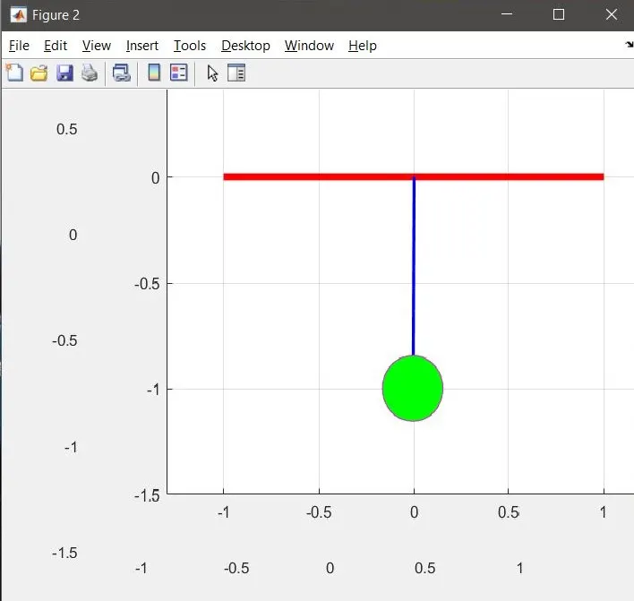
The simulation was done successfully, and the graph of displacement and velocity were plotted successfully as shown below in the pictures. The link to the video in You Tube is as below.

https://youtu.be/x8sqs0k2bFY

Conclusions:

1. The graph were plotted, and the simulation was a success.
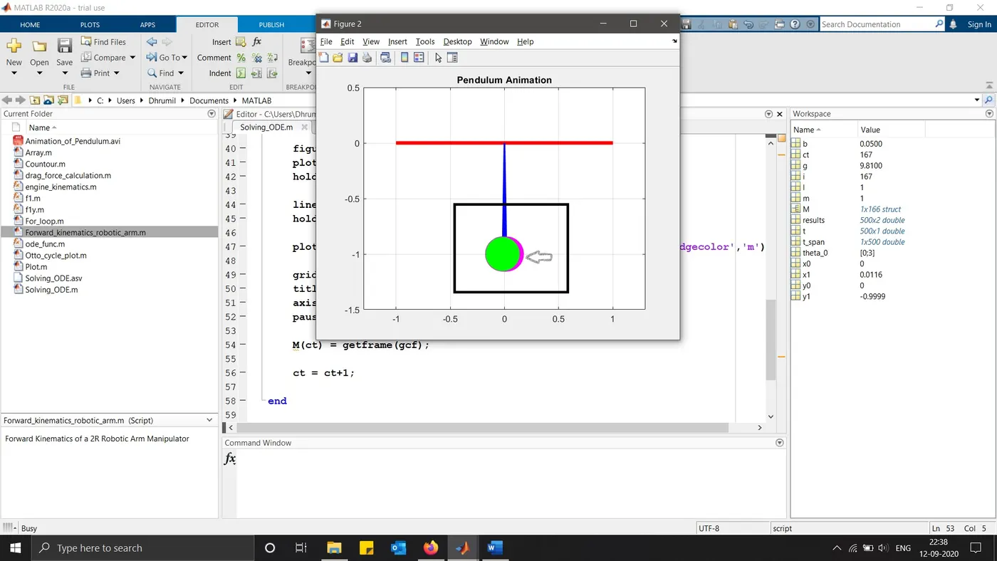
2. There was one difficulty faced as shown below in the picture. As the simulation occurred, the edge of the pendulum sphere was staying at one place where the sphere did not move entirely in a direction defined by the displacement values. Thereafter literature was referred on the internet [2] on the “hold on” command where a function “hold off” was also explained to reset the axis and hence the function “hold off” was experimentally used in the “for loop” where the axis were then reset to a new one every time the sphere oscillated from one position to another. This was a self-learning moment as the pendulum did not simulate as needed.

References:

[1] https://in.mathworks.com/help/matlab/creating_plots/create-line-plot-with-markers.html

[2] http://www.ece.northwestern.edu/local-apps/matlabhelp/techdoc/ref/hold.html

The screenshots of the Matlab window are as follows: