Parsing NASA thermodynamic data using Matlab
Aim:
- To write a Matlab function to extract the 14 coefficients and calculate the enthalpy, entropy, and specific heats for all 53 species in the given THERMO.dat data file.
- To plot the calculated Cp, H and S vs temperature of all 53 species and to dump them into their respective folders at a given location.
- To calculate molecular weights of all 53 species in the THERMO.dat file.
Description:
Parser: In computer terminology, a parser is a program which is usually part of a compiler, that receives input in the form of sequential source program instructions, interactive online commands, mark-up tags, or some other defined interface and breaks them up into parts for example fetching out a particular data from an external file that can then be managed by other programming let’s say plotting the data or calculating necessary things from that data or can be used by another programs for specific necessities. A parser may also check to see that all input has been provided that is necessary [1].
Here for this project we are parsing the available ‘THERMO.dat’ data file released by NASA in 1999 using Matlab, which has thermodynamic data produced by NASA, from which we have to extract the data regarding to temperatures and coefficients related to the 53 species in the data file and hence calculating the Cp (specific heat), Entropy (S) and Enthalpy (H) and later plotting them against temperature and calculating the molecular mass of each of the 53 species.
The formula for calculating Cp, S and H is as shown below
The equation for Specific heat (Cp) is:

The equation for Entropy (S) is:

The equation for Enthalpy (H) is:

Where,
R = Gas Constant
T = Temperature
a1, a2, a3,… a7 = Coefficients
Objectives:
- To write a function to extract 14 coefficients of 53 species.
- To calculate CP, H and S and plot them against temperature range of all 53 species.
- To save the plots of Cp, H and S of each specie in a separate folder, naming the folder according to the species.
- To calculate molecular weight of all 53 species.
- All the above should be done automatically with programming in Matlab.
Theory:
% File parsing. Parsing thermodynamic data by NASA.

clear all
close all
clc

% Reading and opening the "THERMO.dat" file
thermfile = fopen('THERMO.dat','r');
fgetl(thermfile);

% Global Temperatures
temp_line = fgetl(thermfile);
T = strsplit(temp_line,' ');

% Strings to numbers
temp1 = str2num(T{2});
temp2 = str2num(T{3});
temp3 = str2num(T{4});

% To display the global temperature values
head = 'Global Temperature Values are:';
fprintf('%s',head);
disp(temp1);
disp(temp2);
disp(temp3);

% Next three lines are not required
fgetl(thermfile);
fgetl(thermfile);
fgetl(thermfile);

% To read coefficients of each species and further calculations

for i = 1:53
Species = fgetl(thermfile); % Allocating the first line
Species_name = Species(1:6);

% Finding local temperature values for calculations
x = strsplit(Species,' ');
z = length(x);

% Storing the temperature values as numbers
T1 = str2double(x{z-3});
T2 = str2double(x{z-2});
T3 = str2double(x{z-1});

% Local low, high and mid temperatures
Local_low_temp = T1;
Local_high_temp = T2;
Local_mid_temp = T3;


% Reading between the lines to extract the coeffificnets
line2 = fgetl(thermfile); % Allocating second line
l2 = strfind(line2,'E');
a1 = str2num(line2(1:(l2(1)+3)));
a2 = str2num(line2((l2(1)+4):(l2(2)+3)));
a3 = str2num(line2((l2(2)+4):(l2(3)+3)));
a4 = str2num(line2((l2(3)+4):(l2(4)+3)));
a5 = str2num(line2((l2(4)+4):(l2(5)+3)));

line3 = fgetl(thermfile); % Allocating third line
l3 = strfind(line3,'E');
a6 = str2num(line3(1:(l3(1)+3)));
a7 = str2num(line3((l3(1)+4):(l3(2)+3)));
a8 = str2num(line3((l3(2)+4):(l3(3)+3)));
a9 = str2num(line3((l3(3)+4):(l3(4)+3)));
a10 = str2num(line3((l3(4)+4):(l3(5)+3)));

line4 = fgetl(thermfile); % Allocating fourth line
l4 = strfind(line4,'E');
a11 = str2num(line4(1:(l4(1)+3)));
a12 = str2num(line4((l4(1)+4):(l4(2)+3)));
a13 = str2num(line4((l4(2)+4):(l4(3)+3)));
a14 = str2num(line4((l4(3)+4):(l4(4)+3)));

% Tempreatures for calculation
temperature = linspace(Local_low_temp,Local_high_temp,100);

% Gas Constant
R = 8.341;

% Calculations of Cp, H and S based on lower and upper temperatures

  for j = 1:length(temperature)
   if temperature(j)>= Local_mid_temp
       Cp = (a1+a2.*temperature+a3.*temperature.^2+a4.*temperature.^3+a5.*temperature.^4).*R;
       H = (a1+(a2.*temperature)./2+(a3.*temperature.^2)/3+(a4.*temperature.^3)/4+(a5.*temperature.^4)/5+a6./temperature).*temperature.*R;
       S = (a1*log(temperature)+a2.*temperature+(a3.*temperature.^2)/2+(a4.*temperature.^3)/3+(a5.*temperature.^4)/4+a7).*R;
   else
       Cp = (a8+a9.*temperature+a10.*temperature.^2+a11.*temperature.^3+a12.*temperature.^4).*R;
       H = (a8+(a9.*temperature)./2+(a10.*temperature.^2)/3+(a11.*temperature.^3)/4+(a12.*temperature.^4)/5+a13./temperature).*temperature.*R;
       S = (a8*log(temperature)+a9.*temperature+(a10.*temperature.^2)/2+(a11.*temperature.^3)/3+(a12.*temperature.^4)/4+a14).*R;
   end
  end

mkdir(Species_name); % Making a directory to save plots
cd(Species_name); % Current folder to save the plots in respected folders

% Plotting the graphs

% Temperature vs Specific Heat
figure(1)
plot(temperature, Cp, 'linewidth', 2, 'color','r')
xlabel('Temperature [K]')
ylabel('Specific Heat (Cp)')
title(Species_name)

% Temperature vs Enthalpy
figure(2)
plot(temperature, H, 'linewidth', 2, 'color','b')
xlabel('Temperature [K]')
ylabel('Enthalpy (H)')
title(Species_name)

% Temperature vs Entropy
figure(3)
plot(temperature, S, 'linewidth', 2, 'color','m')
xlabel('Temperature [K]')
ylabel('Entropy (S)')
title(Species_name)

% Saving the figures in each folder
saveas(figure(1),'Specific Heat.jpg')
saveas(figure(2),'Enthalpy.jpg')
saveas(figure(3),'Entropy.jpg')

cd ..

% Desplaying molecular weights of all species using the program
% molecular_weight
fprintf('Molecular Weight of the corresponding element: ')
disp(Species_name)
fprintf('is')
molecular_weight(Species_name)

end
% Calculating the molecular weight
function Molecular_weight = molecular_weight(Species_name)
Atoms = {'H';'C';'N';'O';'A'}; % Main atoms
Atomic_weight = [1 12 14 16 40]; % Atomic weights of main atoms
Molecular_weight = 0;
K = split(Species_name,'');
for m = 1:length(Species_name)
for n = 1:(length(Atoms))
if K{m+1}==Atoms{n} % To compare atoms of species with atoms
Molecular_weight = Molecular_weight+Atomic_weight(n);
y=n; % finding the position of particular atoms in the species
end
end
n = str2num(K{m+1}); % for weight of repeating main atoms in the species
if n>1
Molecular_weight = Molecular_weight+Atomic_weight(y)*(n-1);
end
end
end
Explaination of the codes:
% File parsing. Parsing thermodynamic data by NASA.
clear all
close all
clc
% Reading and opening the "THERMO.dat" file
thermfile = fopen('THERMO.dat','r');
fgetl(thermfile);
To start with the program initially a comment was written as a headline for the program saying “% File parsing. Parsing thermodynamic data by NASA.” Thereafter clear all, close all, and clc were written to close clear all the programs running and clear all the data from the workspace window. Then the NASA data file “THERMO.dat” was opened using “fopen” command and therefore was given a command to read the file i.e. “r”. It was assigned to a name “thermfile” which was used further in accessing the file in the program. Command “thermfile = fopen('THERMO.dat','r');” was used to execute the above explained. Thereafter “fgetl(thermfile)” was used to read the characters from the data file, where the first line was of no use which is just the name of the file “THERMO”. Therefore the command “fgetl”.
% Global Temperatures
temp_line = fgetl(thermfile);
T = strsplit(temp_line,' ');
% Strings to numbers
temp1 = str2num(T{2});
temp2 = str2num(T{3});
temp3 = str2num(T{4});
% To display the global temperature values
head = 'Global Temperature Values are:';
fprintf('%s',head);
disp(temp1);
disp(temp2);
disp(temp3);
The above program was written to display the global temperatures in the data file which is the global range of the species in the file. These temperatures varies with species. Where each specie has its own high, low and mid temperature. The global temperature range was extracted for presentation purposes. Therefore to access the second line of the data file the above program was written, which is explained as: The temperature line was allocated to the entity “temp_line” using “fgetl” command to read the line. Thereafter “T” was assigned to the command “strsplit” to split the string according to mentioned entity, here the entity to identify was an empty space therefore the command used was “T = strsplit(temp_line,' ');”. To extract data from any data file, the Matlab recognises the entities as strings and not the numerical values, therefore the command “str2num” is used to convert string arrays to numeric arrays. Here for the Global temperature values, to identify the numbers “str2num” was used to convert the temperature values from strings to numbers. Therefore, three different commands for three values, were written assigned to its name temp1, temp2 and temp3. “temp1 = str2num(T{2});”, “temp2 = str2num(T{3});”, “temp3 = str2num(T{4});” were written to extract numerical temperature values. Thereafter a program was written to display the global temperature values, where the heading was given using “fprintf” command to print the heading line “Global Temperature Values are:” in the command window and thereafter displaying the global temperature values using “disp” command with temp1, temp2 and temp3 values, that were 300, 1000 and 5000.
Thereafter the next three lines were the comments made in the datafile which are of no use in the calculations, that can be ignored using “fgetl” command which is shown below.
% Next three lines are not required
fgetl(thermfile);
fgetl(thermfile);
fgetl(thermfile);
Starting to fetch the coefficients of each species and fetching the local temperature values of each species the further commands were used using “for loop” in the command, the “for loop” was used in order to do the calculations simultaneously which only stops when all the calculations for the species were done including plotting the graphs for Cp, S and H against temperature values of each species. There are in total 53 species for which the calculations were carried out simultaneously. Therefore, starting with the below commands with its explanation.
% To read coefficients of each species and further calculations
for i = 1:53
Species = fgetl(thermfile); % Allocating the first line
Species_name = Species(1:6);
% Finding local temperature values for calculations
x = strsplit(Species,' ');
z = length(x);
% Storing the temperature values as numbers
T1 = str2double(x{z-3});
T2 = str2double(x{z-2});
T3 = str2double(x{z-1});
Local_low_temp = T1; % Local low, high and mid temperatures
Local_high_temp = T2;
Local_mid_temp = T3;
Firstly “i” was given for the starting of the “for loop” for 53 species, then the species name were identified using the “fgetl” command and assigning the first line to “Species”, thereafter the characters of the name of all the species were recognised by the command “Species” which extracts the letters of the species from the data file, therefore the command “Species_name = Species(1:6);” was used to extract species name which was assigned to the name “Species_name” for the further use of the word. As seen in the datafile, maximum number of letters in all the species is no more than 6 letters therefore “(1:6)” that is letters 1 to 6 were extracted to name the species.
After extracting the species name, local temperatures were extracted of all the species where a comment “% Finding local temperature values for calculations” was written to identify the purpose of the code written. An “x” was assigned to identify the line of the local temperatures and identify the empty spaces in the line “x = strsplit(Species,' ');”, this is the same line used to identify the species name therefore “Species” line was used to identify the temperatures in the same line, thereafter “z” was assigned to the “length” of the line “x” by writing the command “z = length(x);”.
Thereafter the commands were written to store the local temperature values for each species and identifying the numbers using the “str2double” command to accurately identify the numeric values in the respective line. Therefore T1, T2 and T3 were assigned to low, high and middle local temperatures. By writing the commands “T1 = str2double(x{z-3});”, “T2 = str2double(x{z-2});”, “T3 = str2double(x{z-1});”, where z-1, z-2 and z-3 are the locations of the temperature values which had to be given in curly brackets, where “z” is assigned as the length of line “x”. Thereafter, T1, T2 and T3 were named as “Local_low_temp”, “Local_high_temp” and “Local_mid_temp” respectively for further calculations of CP, S and H.
After identifying and extracting the temperature values, the 14 coefficients of all the 53 species had to be extracted and to identify and extract all 14 coefficients, the following codes were written, which is explained below.
% Reading between the lines to extract the coefficients
line2 = fgetl(thermfile); % Allocating second line
l2 = strfind(line2,'E');
a1 = str2num(line2(1:(l2(1)+3)));
a2 = str2num(line2((l2(1)+4):(l2(2)+3)));
a3 = str2num(line2((l2(2)+4):(l2(3)+3)));
a4 = str2num(line2((l2(3)+4):(l2(4)+3)));
a5 = str2num(line2((l2(4)+4):(l2(5)+3)));
line3 = fgetl(thermfile); % Allocating third line
l3 = strfind(line3,'E');
a6 = str2num(line3(1:(l3(1)+3)));
a7 = str2num(line3((l3(1)+4):(l3(2)+3)));
a8 = str2num(line3((l3(2)+4):(l3(3)+3)));
a9 = str2num(line3((l3(3)+4):(l3(4)+3)));
a10 = str2num(line3((l3(4)+4):(l3(5)+3)));
line4 = fgetl(thermfile); % Allocating fourth line
l4 = strfind(line4,'E');
a11 = str2num(line4(1:(l4(1)+3)));
a12 = str2num(line4((l4(1)+4):(l4(2)+3)));
a13 = str2num(line4((l4(2)+4):(l4(3)+3)));
a14 = str2num(line4((l4(3)+4):(l4(4)+3)));
A starting comment “% Reading between the lines to extract the coefficients” was written to recognise what code was written. Here in the data file, each species has a total of four line where:
First line: Has the species name and the local temperature values
Second line: Has total of 5 coefficients with a letter “E” in between indicating the power to that specific coefficient.
Third line: Has total of 5 coefficients with a letter “E” in between indicating the power to that specific coefficient.
Fourth line: Has a total of 4 coefficients with a letter “E” in between indicating the power to that specific coefficient.
Here in this case, similar to identifying the temperature values with the help of blank spaces, here we can identify the coefficient values by locating and analysing the location of “E” in the line and extract the coefficient values of the species. To extract the coefficient values, we need to know the total numbers of numerals before “E” and after “E”. Therefore, the code to analyse the location of “E”, the command “l2 = strfind(line2,'E');” was used where line number two was assigned to the entity “line2” in the commands, where”line2” was assigned to allocate the second line of the total four lines that we analysed for a single species, the command “ line2 = fgetl(thermfile);” was written to allocate the second line after the first line.
Thereafter, coefficients a1, a2, a3, a4 and a5 were extracted using “str2num” that converts the sting array to numeric array, and by locating the numeric values by locating “E” where letter ”E” is stored in the form “l2” command, in the first line by writing the commands “a1 = str2num(line2(1:(l2(1)+3)));”, “a2 = str2num(line2((l2(1)+4):(l2(2)+3)));”, “a3 = str2num(line2((l2(2)+4):(l2(3)+3)));”, “a4 = str2num(line2((l2(3)+4):(l2(4)+3)));” and “a5 = str2num(line2((l2(4)+4):(l2(5)+3)));”.
Similarly, coefficients a6, a7, a8, a9, a10, a11, a12, a13 and a14 were extracted by locating third and fourth lines in the program, where in fourth line there were only four coefficients.
After extracting the coefficients of the species, the value of universal gas constant “R” was defined in the program. Thereafter, the temperature values were divided into 100 parts ranging from low temperature value to high temperature value. The code for the same is as shown below.
% Tempreatures for calculation
temperature = linspace(Local_low_temp,Local_high_temp,100);
% Gas Constant
R = 8.341;
After that, the calculations of Cp, S and H were done by writing the following code.
% Calculations of Cp, H and S based on lower and upper temperatures
for j = 1:length(temperature)
if temperature(j)>= Local_mid_temp
Cp = (a1+a2.*temperature+a3.*temperature.^2+a4.*temperature.^3+a5.*temperature.^4).*R;
H = (a1+(a2.*temperature)./2+(a3.*temperature.^2)/3+(a4.*temperature.^3)/4+(a5.*temperature.^4)/5+a6./temperature).*temperature.*R;
S = (a1*log(temperature)+a2.*temperature+(a3.*temperature.^2)/2+(a4.*temperature.^3)/3+(a5.*temperature.^4)/4+a7).*R;
else
Cp = (a8+a9.*temperature+a10.*temperature.^2+a11.*temperature.^3+a12.*temperature.^4).*R;
H = (a8+(a9.*temperature)./2+(a10.*temperature.^2)/3+(a11.*temperature.^3)/4+(a12.*temperature.^4)/5+a13./temperature).*temperature.*R;
S = (a8*log(temperature)+a9.*temperature+(a10.*temperature.^2)/2+(a11.*temperature.^3)/3+(a12.*temperature.^4)/4+a14).*R;
end
endHere in the calculations a “for loop” is used with “j” define to the length of temperature and an “if” condition is applied between high temperature coefficients and low temperature coefficients, where if the temperature is greater than the middle temperature it will take first 7 coefficients a1 to a7 and if the temperature is lesser than the middle temperature it will take the other 7 coefficients a8 to a14 for the calculations of CP, S and H with the formulas shown before in the description.
After the calculations of CP, S and H, for all the species, the graphs of “Temperature vs Cp”, “Temperature vs S” and “Temperature vs H” were plotted using the following commands. Before writing commands to plot the graphs, a “mkdir” command was written to make a directory to save the plots in different folders as the name of species with their three plots in that folder respectively writing the command as “mkdir(Species_name)” where the command will create a folder with the species name on it [2]. Thereafter, the “cd” command was given to change the directory to the current directory with species name. After the plot commands a command “cd ..” was given to determine that it was the one level upper of the current folder that we are saving the graphs in [3]. The commands given to plot and save the graphs are as below.
mkdir(Species_name); % Making a directory to save plots
cd(Species_name); % Current folder to save the plots in respected folders
% Plotting the graphs
% Temperature vs Specific Heat
figure(1)
plot(temperature, Cp, 'linewidth', 2, 'color','r')
xlabel('Temperature [K]')
ylabel('Specific Heat (Cp)')
title(Species_name)
% Temperature vs Enthalpy
figure(2)
plot(temperature, H, 'linewidth', 2, 'color','b')
xlabel('Temperature [K]')
ylabel('Enthalpy (H)')
title(Species_name)
% Temperature vs Entropy
figure(3)
plot(temperature, S, 'linewidth', 2, 'color','m')
xlabel('Temperature [K]')
ylabel('Entropy (S)')
title(Species_name)
% Saving the figures in each folder
saveas(figure(1),'Specific Heat.jpg')
saveas(figure(2),'Enthalpy.jpg')
saveas(figure(3),'Entropy.jpg')
cd ..
The “plot” command was used to plot the graphs and one more command was used to save each plot in the respective directory was “saveas” which in default is “saveas(fig,filename)”, was written separately for all three graphs to individually save the plots in the respective folder and naming the plots as “Specific Heat.jpg” “Enthalpy.jpg” and “Entropy.jpg”. Therefore figure(1) was saved as Specific Heat, because the command for figure 1 was to plot Temperature vs Specific Heat, figure(2) was saved as Enthalpy, because the command for figure 2 was to plot Temperature vs Enthalpy and figure(3) was saved as Entropy, because the command for figure 3 was to plot Temperature vs Entropy, in the species folders. The screenshot of all the saved folders is shown in the end of this report and as per the requirements, the plots of O2, N2 and CO2 are shown in the results section.
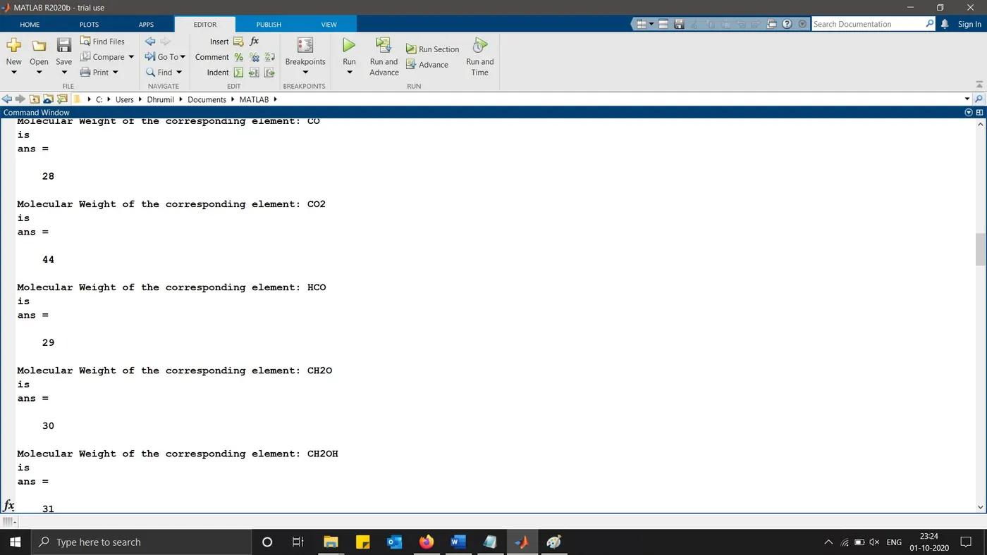
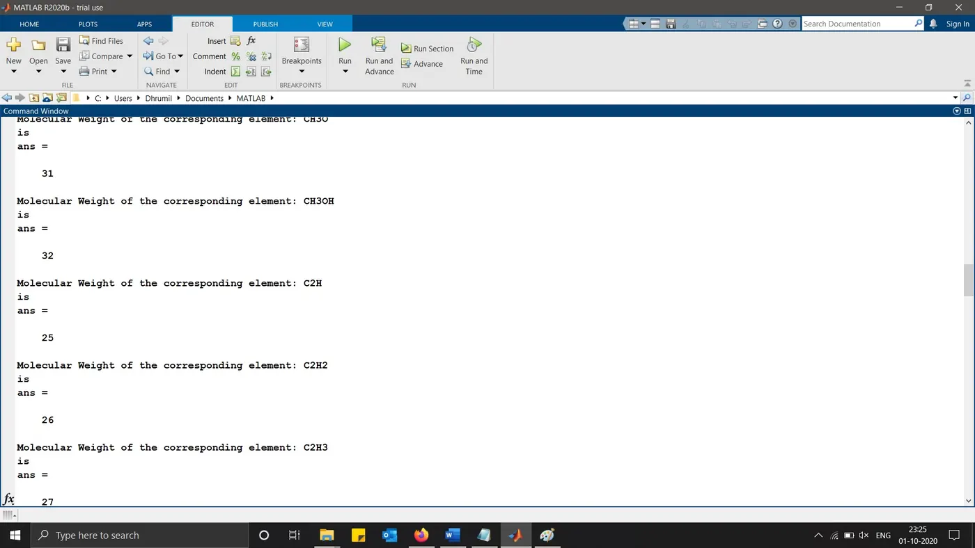
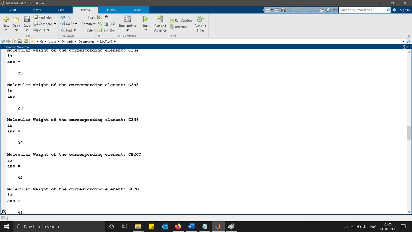
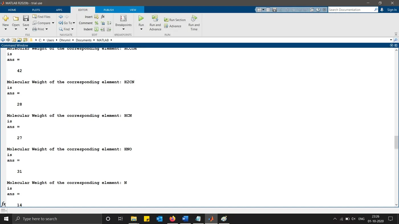
After plotting the graphs of CP, S and H, the molecular weight of all the species were calculated using a function written for calculation and therefore calling that function in the main program and thereafter displaying the calculated molecular weights in the command window. The commands written to display the molecular weights of all the species was written as shown below.
% Desplaying molecular weights of all species using the program
% molecular_weight
fprintf('Molecular Weight of the corresponding element: ')
disp(Species_name)
fprintf('is')
molecular_weight(Species_name)
endHere in this code, the function created to calculate the molecular weights is called as “molecuale_weight(Species_name)”, the function code written to calculate the molecular weight is as shown below. The command “fprintf” was written to print the statement saying “'Molecular Weight of the corresponding element: “ and then followed by displaying the name of the corresponding species and then the answer to display the calculated molecular weight of that specific species by calling the “molecuale_weight” function.
% Calculating the molecular weight
function Molecular_weight = molecular_weight(Species_name)
Atoms = {'H';'C';'N';'O';'A'}; % Main atoms
Atomic_weight = [1 12 14 16 40]; % Atomic weights of main atoms
Molecular_weight = 0;
K = split(Species_name,'');

for m = 1:length(Species_name)
    for n = 1:(length(Atoms))

        if K{m+1}==Atoms{n} % To compare atoms of species with atoms
            Molecular_weight = Molecular_weight+Atomic_weight(n);
            y=n; % finding the position of particular atoms in the species
        end
    end
    n = str2num(K{m+1}); % for weight of repeating main atoms in the species
    if n>1
        Molecular_weight = Molecular_weight+Atomic_weight(y)*(n-1);
    end
end
end
Here to calculate the molecular weight of all the 53 species, the main atoms of the species were analysed namely: Hydrogen (H), Carbon (C), Nitrogen (N), Oxygen (O) and Argon (A), following by their atomic weights 1, 12, 14, 16 and 40 respectively. These entities were assigned to the names “Atoms” and “Atomic_weight”. Thereafter a for loop was used to calculate molecular weight of each species and will only stop when calculations has been done for all species, hence including this function in the main command. Initially the molecular weight was taken as 0 and then “K” was defined to analyse the atom in each species and to calculate the molecular weight by writing “K = split(Species_name,'');”. At the start of the for loop “m” was defined as the length of all the species thereafter “n” was defined as the length of the number of atoms, then to compare the atoms of species with the base atoms, an “if” condition was applied that if the number of atoms in the species is equal to the name of atom then the molecular weight formula used was “Molecular_weight = Molecular_weight+Atomic_weight(n);” and then allocating “y” which was equal to “n” to find the position of the particular atom in the species. A second “if” condition was used to determine if that particular atom was repeating in the species which is if “n>1”, then the formula used was “Molecular_weight = Molecular_weight+Atomic_weight(y)*(n-1);”. Thereafter the “if” condition was ended and “for” loop for the function was ended. Thereafter the function was called in the master code to display the calculated molecular weights of all 53 species.
At the end of the master code for parsing the file the code was ended with the "end" for the "for loop" started to calculate the CP, S and H of species.
Results:
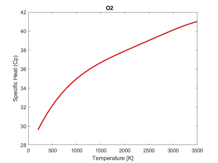
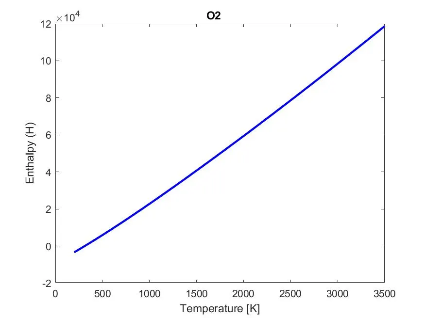
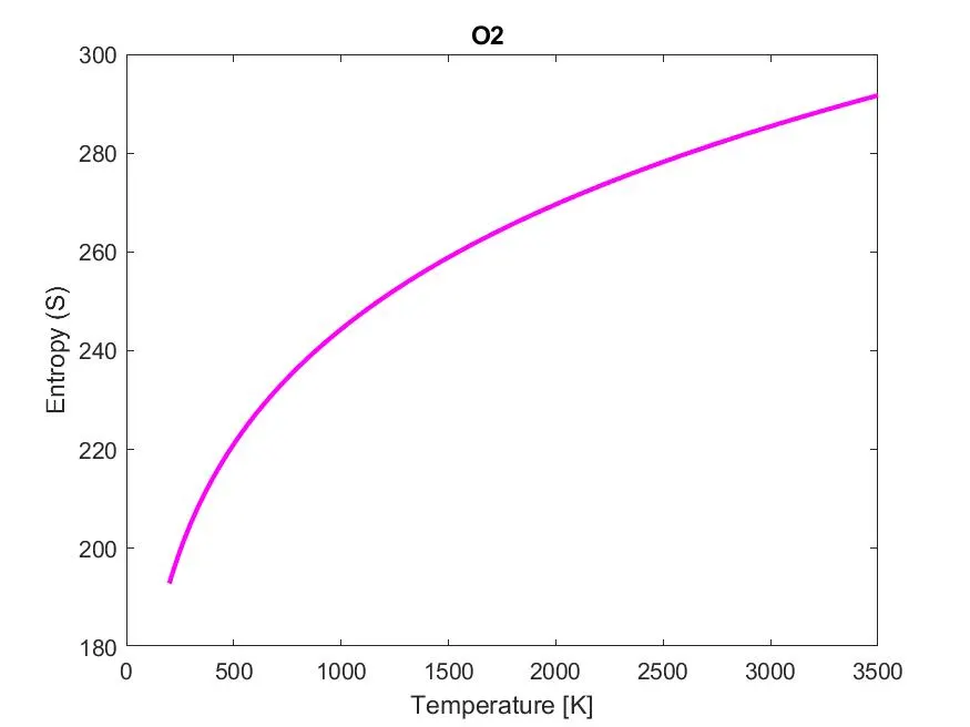
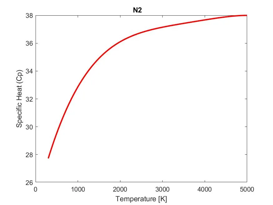
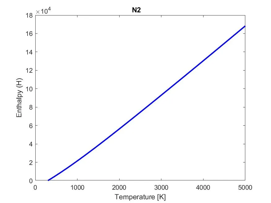
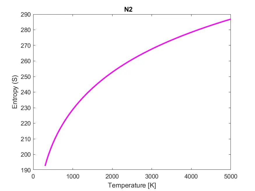
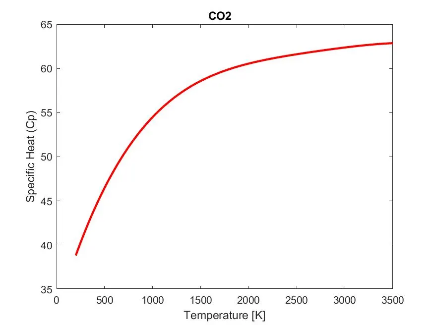
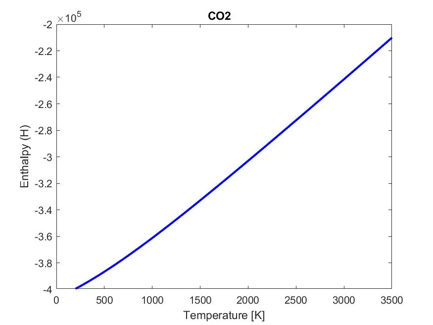
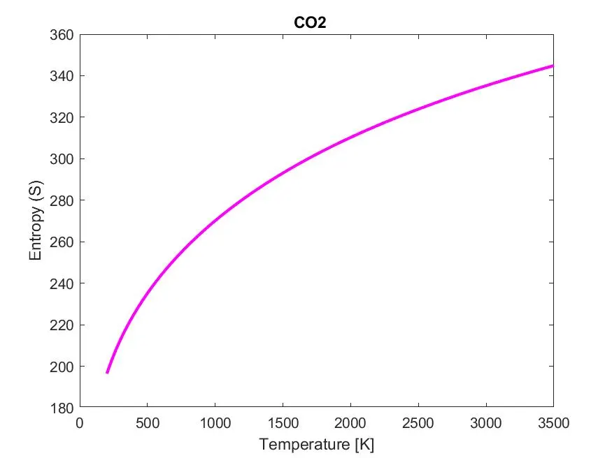
- The Temperature vs Specific Heat, Temperature vs Enthalpy and Temperature vs Entropy plots of O2, N2 and CO2 are shown below.
- The nature of graph of enthalpy seen in the plots is the linear positive slope where, when the temperature increases the enthalpy of the species is increasing. Where enthalpy is a thermodynamic quantity that is equal to total heat content of the system, it is a sum of the internal energy and the product of pressure and volume of a system.
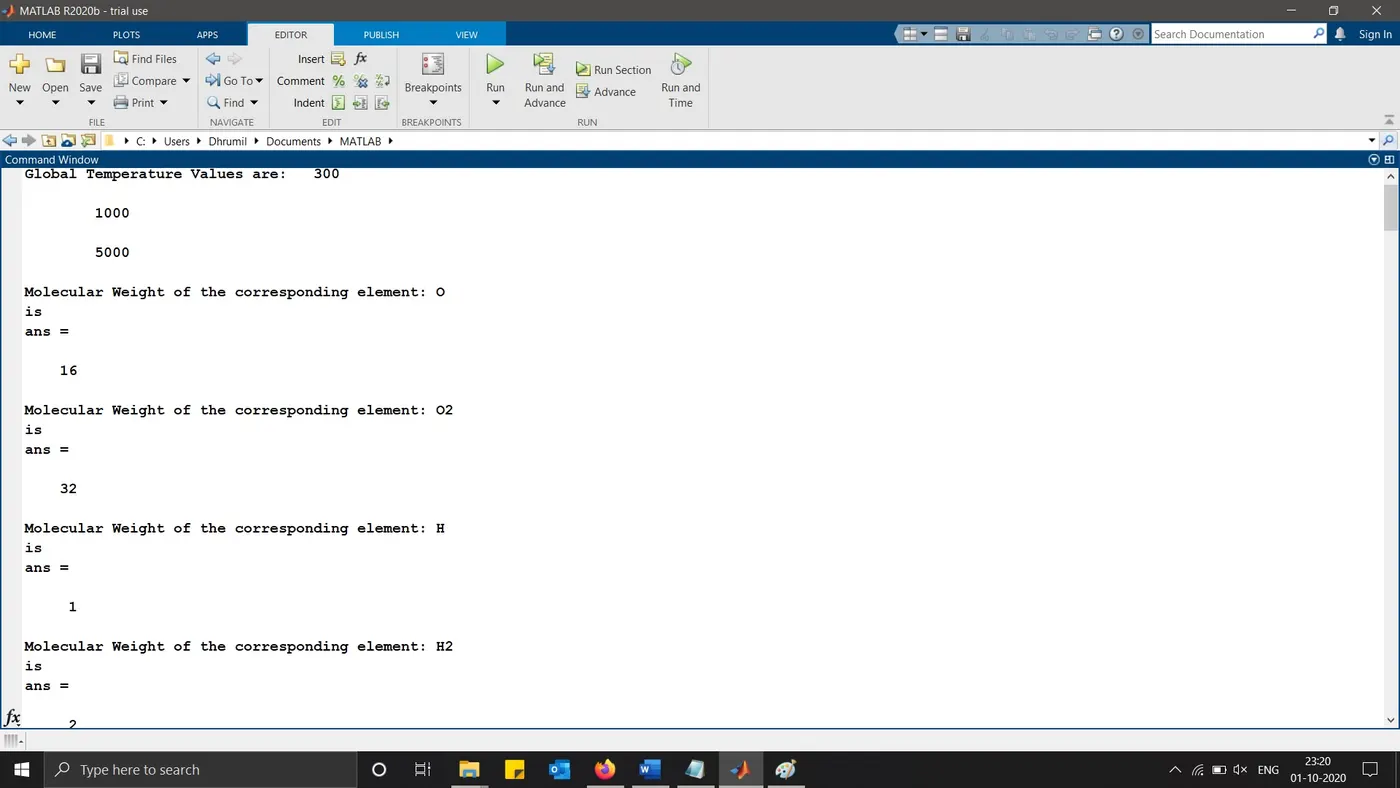
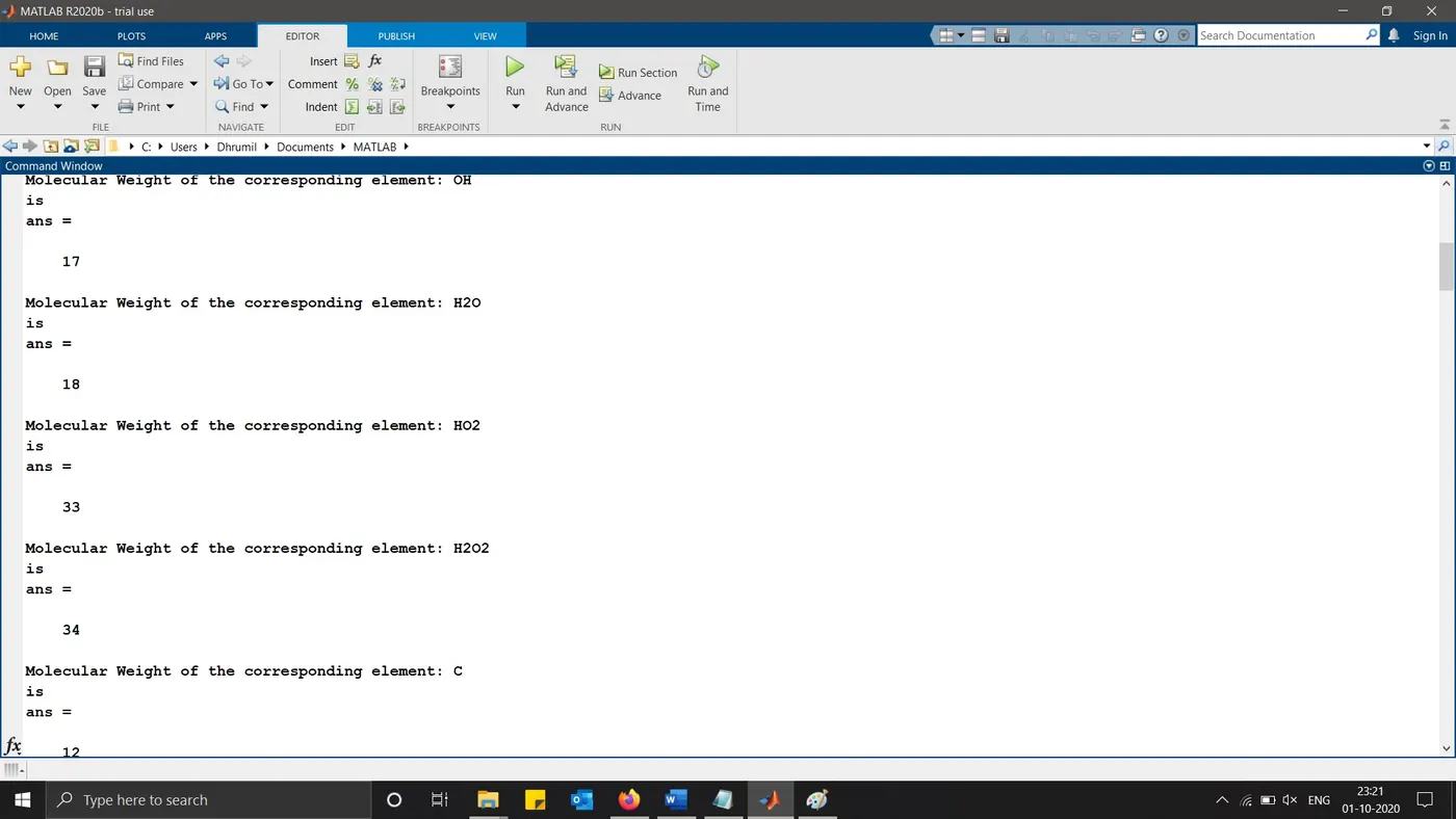
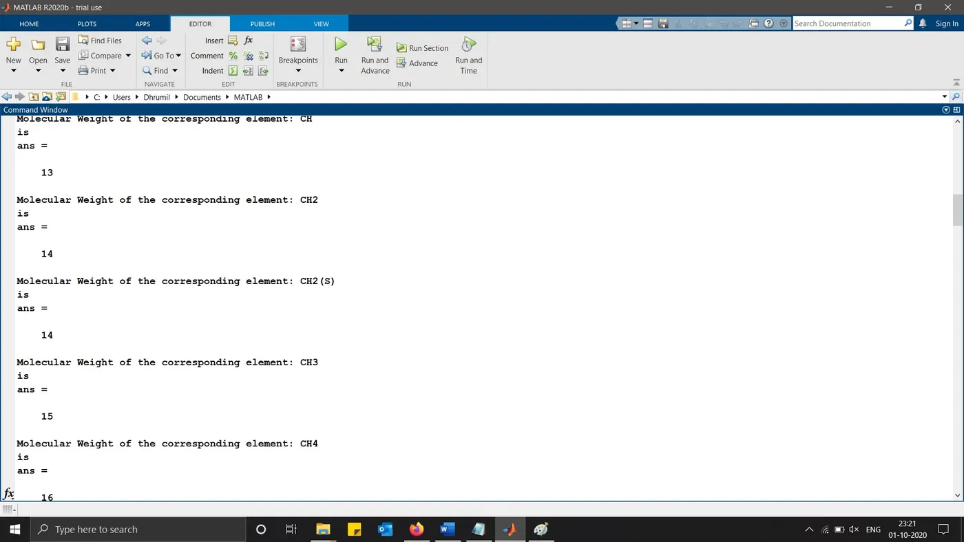
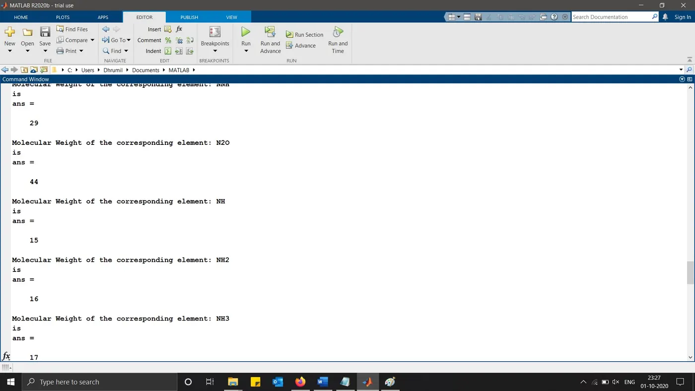
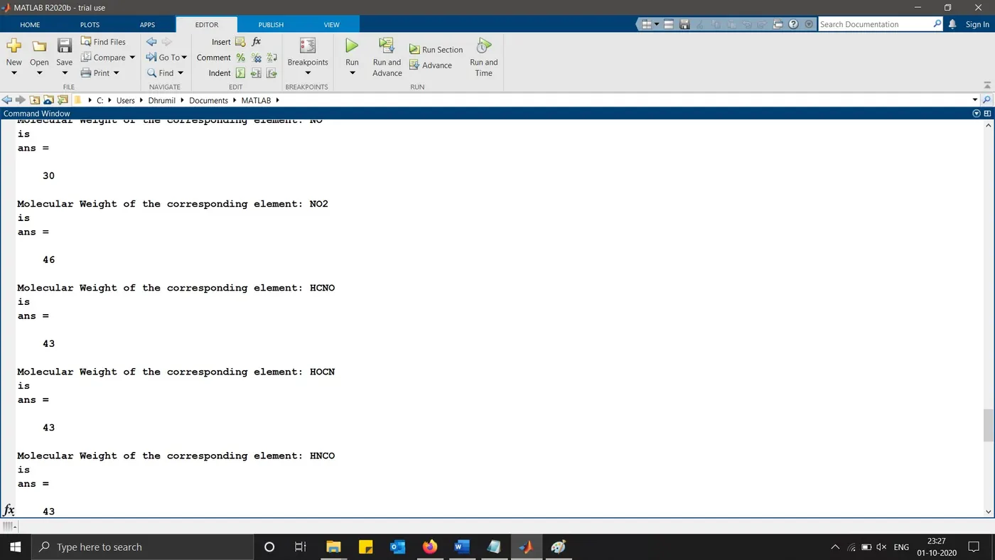
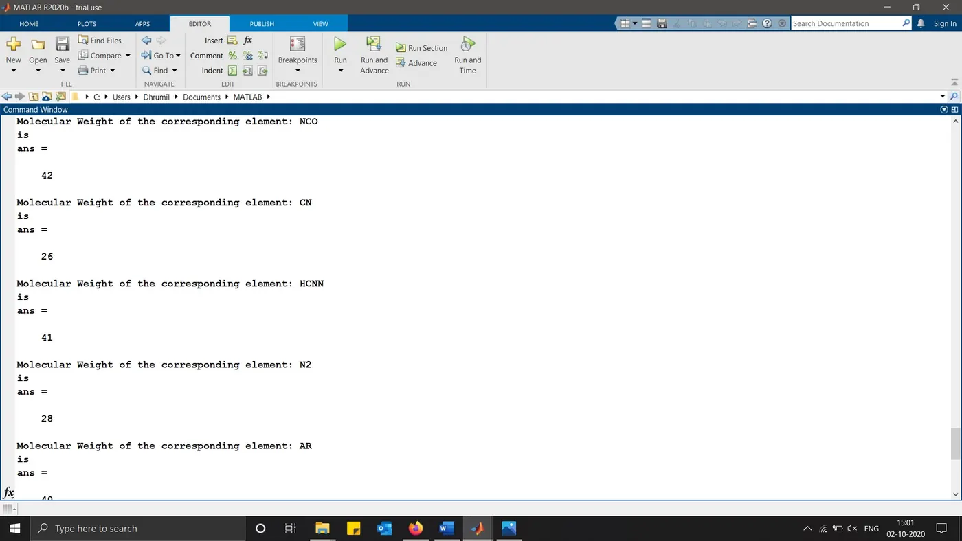
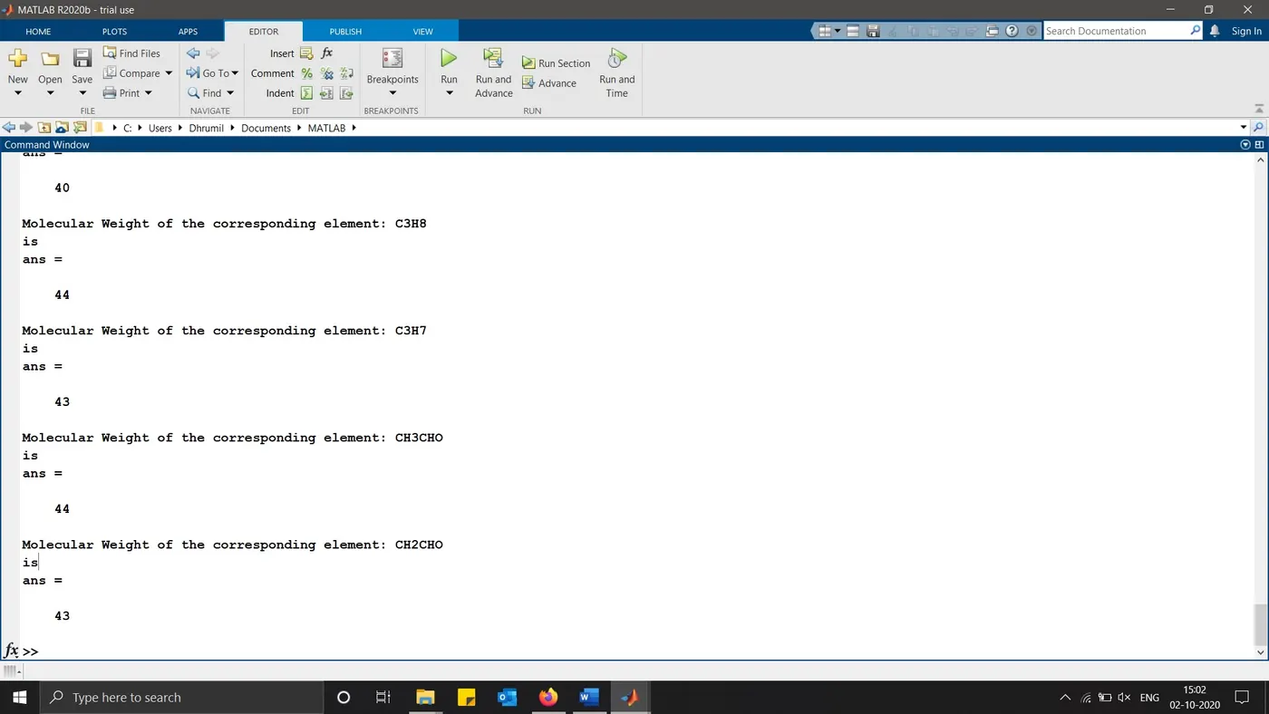
- The molecular weight in the command window are shown below.
Cp, H and S plots of O2:
Cp, H and S plots of N2:
Cp, H and S plots of CO2:
Screenshot of saved folders:

Screenshots of molecular weights of the species:
Errors faced:
There were multiple errors faced during executing the program, the errors are listed below.
1) Loop and Character Error
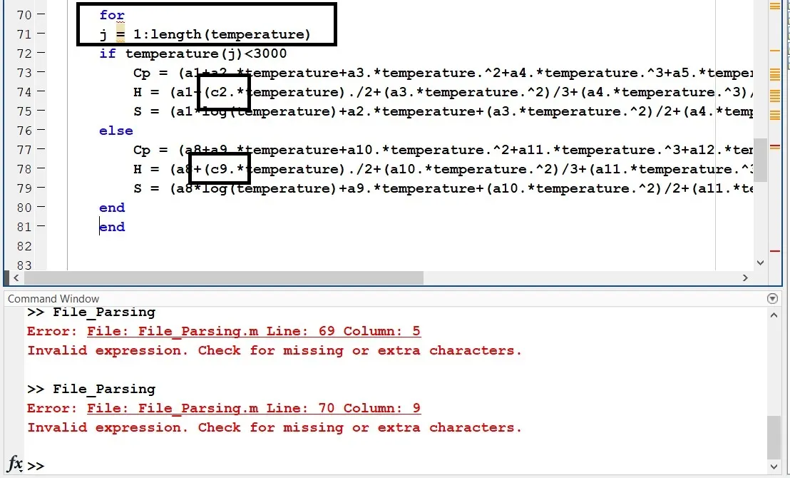
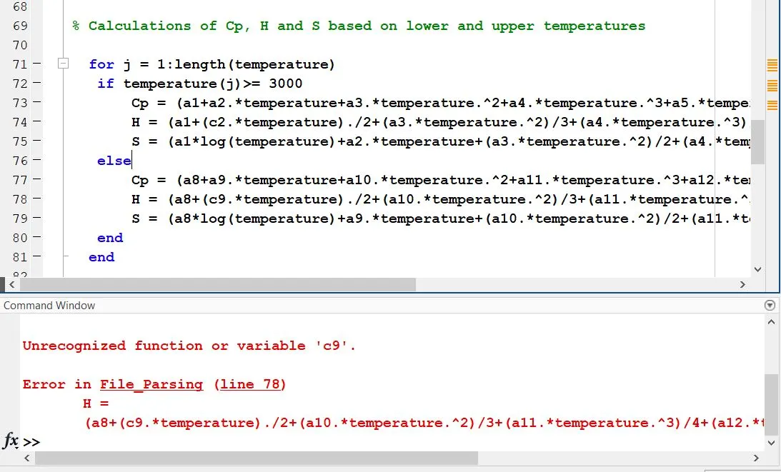
The above error occurred by not using the “for loop” correctly, where “for j=1:length(temperature)” should be in one line. This error was rectified when the error was occurring in the command window and then by looking at the other codes written for “for loop” and then was corrected. However, after rectifying the loop error another error experienced was the wrong character typed in the command which is “c” in the place of “a” which is allocated to fetch the coefficient of the species. Also, the temperature range used was wrong, which was rectified when the local temperatures were extracted.
2) Error while extracting Local Temperature values.
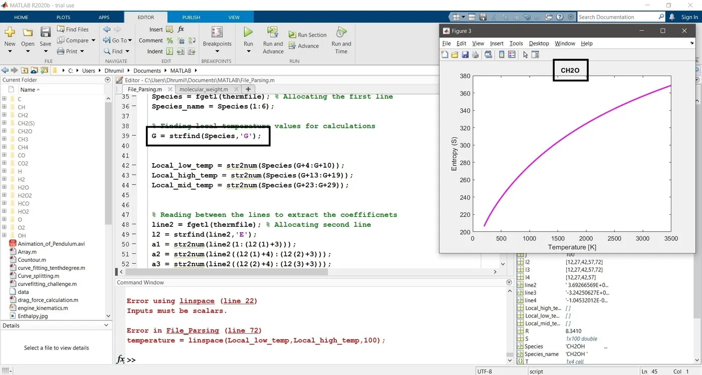
Another error faced was while extracting the values of local temperature when the program detected more than one “G” in the local temperature line and the method to extract local temperatures was considered wrong. It was initially assumed that there will be only one “G” in the line of local temperatures, however, when looked through the document there were more than one G, therefore the program was getting stopped after plotting CH2O plots as shown in the figure below of the data file CH2OH had two G in the line of temperature.
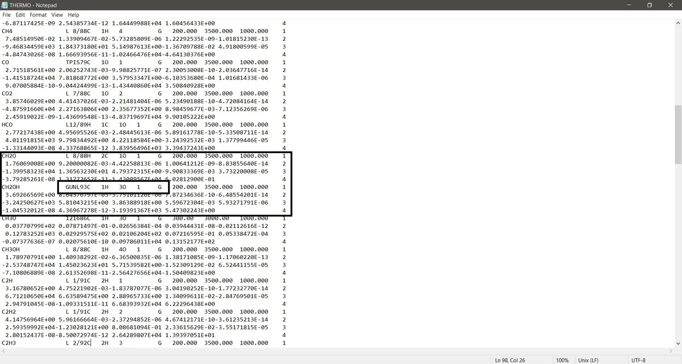
The code for extracting the local temperatures was changed wholly and another method was used to extract the temperatures, by using the code “length” of the whole line and then to fetch the numerical values which can be seen in the main code.
3) Error using ^ sign in Enthalpy formulae.
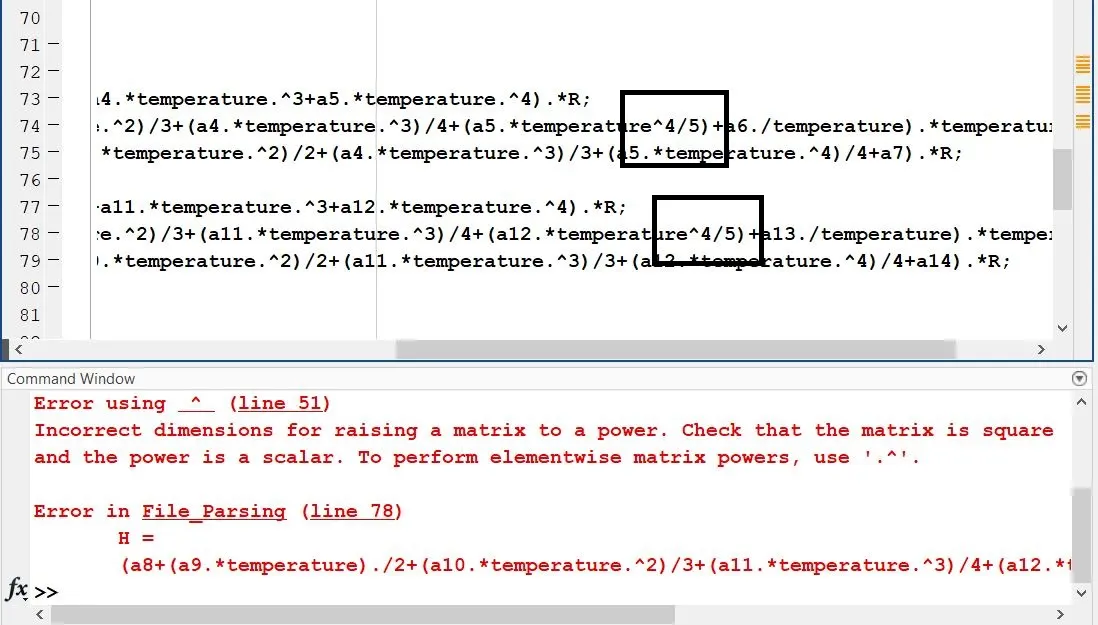
The error was faced while not using a “.” for the temperature input in the Enthalpy equation. This was then rectified by going to the line and rechecking the expressions used in the formulae.
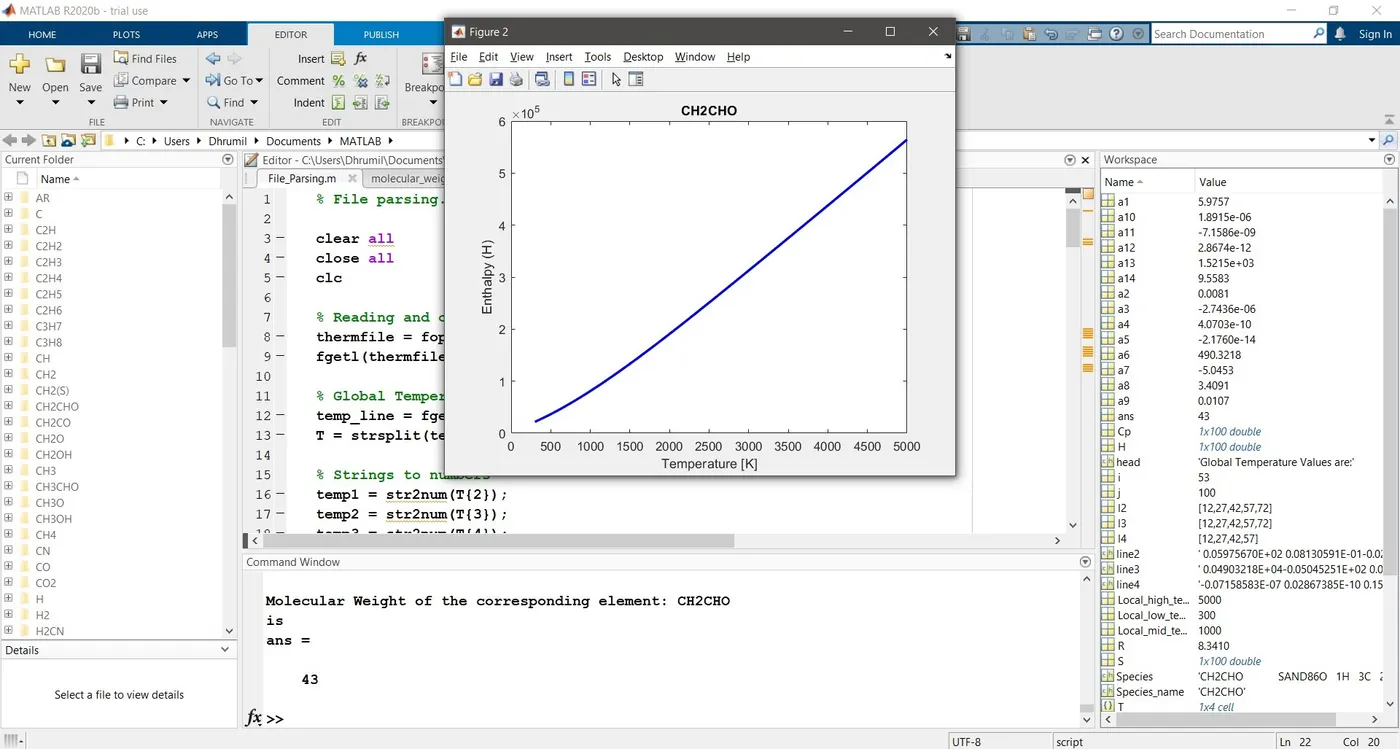
Matalb window screenshot:
References:
[1] https://searchapparchitecture.techtarget.com/definition/parser
[2] https://in.mathworks.com/help/matlab/ref/mkdir.html?s_tid=srchtitle
[3] https://in.mathworks.com/help/matlab/ref/cd.html?s_tid=srchtitle