Optimization of stalagmite function using Genetic Algorithm

Aim:

1. Write a code in Matlab to optimise the stalagmite function and find the global maxima of the function.
2. To explain the concept of genetic algorithm and explain the syntax for ‘ga’ in Matlab.

Description:

Stalagmite:

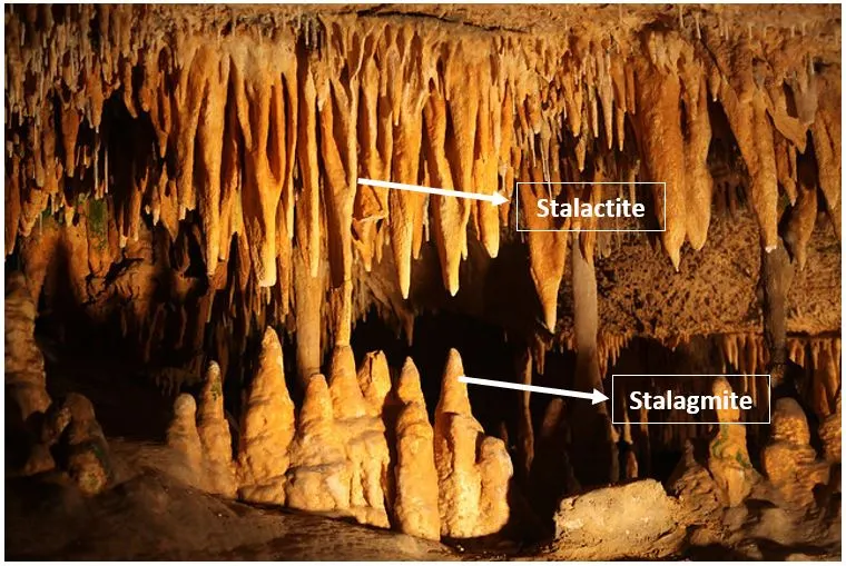
It is an elongated form of various minerals deposited from solution by slowly dripping water. A stalactite hangs like an icicle from the ceiling or sides. A stalagmite appears like an inverted stalactite, rising from the floor. As shown in the picture below. Here in this project stalagmite is used to elaborate the use of “GA” in finding the maximas and minimas.

Genetic Algorithm:

A genetic algorithm is a search investigative that was inspired by Charles Darwin’s theory of natural evolution. It is a technique that is used to solve non-linear optimization problems. Genetic algorithm reflects the process of natural selection where the fittest individuals are selected for reproduction in order to produce offspring of the next generation. This concept is used to find the global minima to optimize the problem. Successive generations evolves through the processes that are mentioned below.

As shown in the figure below, the evolutionary generational cycle works as a group of search and optimization engines inspired by the natural processes of evolution. Evolutionary algorithms uses the evolutionary selection, variation, and replacement operations to augment or replace populations in a generational manner in order to improve the overall fittest solution [1].

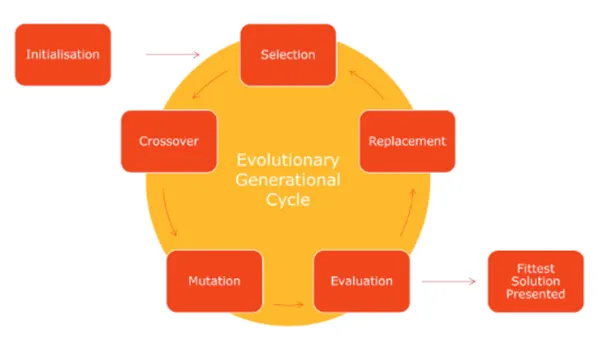
The genetic algorithm works in the following steps.

1. The genetic algorithm begins by creating a random initial population
2. It then creates a sequence of new populations, then at every step it uses the current generation to create next population. To create a new population the algorithm does the following steps.
   1. Rates each member of the population by computing its fitness. That is known as fitness score.
   2. Then it rates the raw fitness scores to convert them into operational values, which are known as expectation values.
   3. Then it selects the members and parents based on the expectations.
   4. Some members who have lower fitness in the current population, are passed on to the next population, which are chosen as elite members.
   5. It then produces new children from the parents by making random changes to a single parent i.e. mutation or by combining the vector entries of the parent pair i.e. crossover.
3. The algorithm then stops when the one of the stopping criteria is met [2]

The GA stops when, after a predefined number of generations or if some stopping criterion has been met for example the fitness above the threshold or if the error rate is below any threshold. The fittest solution in the population is then returned as the global best solution.

GA syntax in Matlab: The GA syntaxes as described in [3] are:

x = ga(fun,nvars)

x = ga(fun,nvars,A,b)

x = ga(fun,nvars,A,b,Aeq,beq)

x = ga(fun,nvars,A,b,Aeq,beq,lb,ub)

x = ga(fun,nvars,A,b,Aeq,beq,lb,ub,nonlcon)

x = ga(fun,nvars,A,b,Aeq,beq,lb,ub,nonlcon,options)

x = ga(fun,nvars,A,b,[],[],lb,ub,nonlcon,IntCon)

x = ga(fun,nvars,A,b,[],[],lb,ub,nonlcon,IntCon,options)

x = ga(problem)

[x,fval] = ga(___)

[x,fval,exitflag,output] = ga(___)

[x,fval,exitflag,output,population,scores] = ga(___)

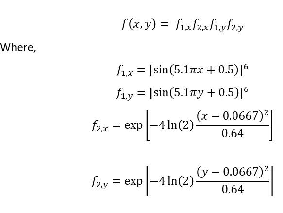
Not all of the syntaxes were used in the project. Only “x = ga(fun,nvars)”, “x = ga(fun,nvars,A,b)” and “x = ga(fun,nvars,A,b,Aeq,beq,lb,ub,nonlcon,options)” were used to program the genetic algorithm using stalagmite function. The stalagmite function was coded using the following formulae:

Theory:

Stalagmite Function:

function [f] = stalagmite_func(input_vector)

x = input_vector(1);
y = input_vector(2);

a = (sin(5.1*pi*x + 0.5))^6;

b = (sin(5.1*pi*y + 0.5))^6;

c = exp(-4*log(2)*((x-0.0667)^2/0.64));

d = exp(-4*log(2)*((y-0.0667)^2/0.64));

f = -a*b*c*d;
end

GA Code:

% To optimise the stalagmite function using Matlab

clear all
close all
clc

% Defining search space

x = linspace(0,0.6,150);
y = linspace(0,0.6,150);


[xx yy] = meshgrid(x, y);

% Evaluating Stalagmite

for i = 1:length(xx)
    
    for j = 1:length(yy)
        
        input_vector(1) = xx(i,j);
        
        input_vector(2) = yy(i,j);
        
        f(i,j) = stalagmite_func(input_vector);
        
    end
end

num_cases = 50;

tic
% Study of Unbounded Inputs: Case 1
for e = 1:num_cases
    
    [inputs, fopt(e)] = ga(@stalagmite_func,2);
    xopt(e) = inputs(1);
    yopt(e) = inputs(2);
end
case_time_Case1 = toc

figure(1)
subplot(2,1,1)
surfc(xx,yy,-f)
xlabel('x values')
ylabel('y values')
shading interp
colorbar
hold on
plot3(xopt,yopt,-fopt,'marker','o','markersize',5,'markerfacecolor','g')
title('Unbound Inputs')
xlabel('x axis')
ylabel('y axis')   

subplot(2,1,2)
plot(fopt)
xlabel('Iteration number')
ylabel('Function Maxima')

num_cases = 50;
tic
% Study of bounding the input values of x and y upper and lower limits
% from 0 to 1: Case 2

for k = 1:num_cases
    [inputs, fopt(k)] = ga(@stalagmite_func, 2, [],[],[],[],[0 0],[1 1]);
    xopt(k) = inputs(1);
    yopt(k) = inputs(2);
end
case_time_Case2 = toc

figure(2)
subplot(2,1,1)
surfc(xx,yy,-f)
xlabel('x values')
ylabel('y values')
shading interp
colorbar
hold on
plot3(xopt,yopt,-fopt,'marker','o','markersize',5,'markerfacecolor','r')
title('Bounded Inputs')
xlabel('x axis')
ylabel('y axis')   

subplot(2,1,2)
plot(fopt)
xlabel('Iteration number')
ylabel('Function Maxima')




num_cases = 50;
tic
% Increasing the GA population to pick the number of optimization, where
% more population means better result: Case 3

options = optimoptions('ga');
options = optimoptions(options,'PopulationSize',350);

for l = 1:num_cases
    [inputs, fopt(l)] = ga(@stalagmite_func, 2, [],[],[],[],[0 0],[1 1],[],[],options);
    xopt(l) = inputs(1);
    yopt(l) = inputs(2);
end
case_time_Case3 = toc

figure(3)
subplot(2,1,1)
surfc(xx,yy,-f)
xlabel('x values')
ylabel('y values')
shading interp
colorbar
hold on
plot3(xopt,yopt,-fopt,'marker','o','markersize',5,'markerfacecolor','k')
title('Optimization with large population')
xlabel('x axis')
ylabel('y axis')   

subplot(2,1,2)
plot(fopt)
xlabel('Iteration number')
ylabel('Function Maxima')

Explanation for Stalagmite function:

As seen in the formulae above, used to code the stalagmite function, there are two input vectors namely x and y. Therefore, two vectors are inserted in the function to take the input values to calculate the stalagmite functions. Hence “x = input_vector(1)” and “y = input_vector(2)” are written at the start of the function. The function for stalagmite formulae is define here in the program as “stalagmite_func”, which is later used in coding further in the GA calculations. In the function the “-“ sign in given to the calculation of the output of the function “f” is to get the global maxima.

Explanation for GA algorithm command:

% To optimise the stalagmite function using Matlab

clear all
close all
clc

% Defining search space

x = linspace(0,0.6,150);
y = linspace(0,0.6,150);

Initially a text was written for the headline of the command giving a % sign to indicate it is a normal text which was “To optimise the stalagmite function using Matlab”. Thereafter commands to clear the command space and to stop any running command was given. The input values for x and y vectors were defined between 0 and 0.6 which was divided into 150 random values.

[xx yy] = meshgrid(x, y);

% Evaluating Stalagmite

for i = 1:length(xx)
    
    for j = 1:length(yy)
        
        input_vector(1) = xx(i,j);
        
        input_vector(2) = yy(i,j);
        
        f(i,j) = stalagmite_func(input_vector);
        
    end
end

Thereafter, the command “meshgrid” was used to create a 2D array. Thereafter the “for loop” method was used and stalagmite function was called inside the loop to calculate the “f” where input vectors were x and y, where “i” and “j” were defined as from 1 to length of xx and yy which were output arrays of x and y array when we created a 2D array of x and y values.

Programming for Case 1, Unbounded inputs:

num_cases = 50;
tic
% Study of Unbounded Inputs: Case 1
for e = 1:num_cases
    
    [inputs, fopt(e)] = ga(@stalagmite_func,2);
    xopt(e) = inputs(1);
    yopt(e) = inputs(2);
end
case_time_Case1 = toc

figure(1)
subplot(2,1,1)
surfc(xx,yy,-f)
xlabel('x values')
ylabel('y values')
shading interp
colorbar
hold on
plot3(xopt,yopt,-fopt,'marker','o','markersize',5,'markerfacecolor','g')
title('Unbound Inputs')
xlabel('x axis')
ylabel('y axis')   

subplot(2,1,2)
plot(fopt)
xlabel('Iteration number')
ylabel('Function Maxima')

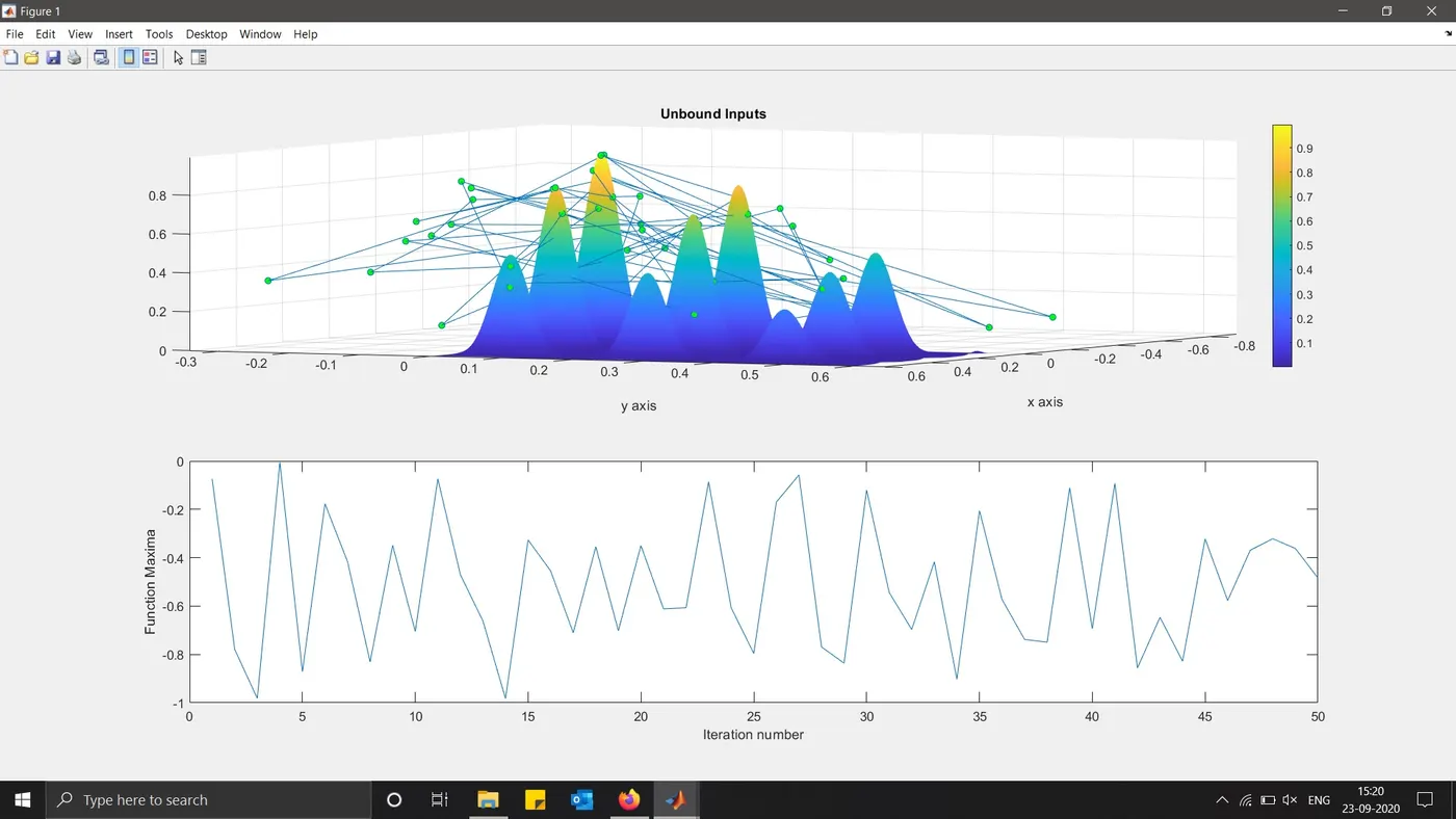
In this case, where the inputs were unbounded, no specific inputs were defined to the GA in stalagmite function. Here the GA syntax “x = ga(fun,nvars)” was used in the loop to study the unbounded inputs. Where “fun” was the stalagmite function previously coded and this GA syntax finds a local unconstrained minimum, x, to the objective function, “stalagmite_func”. And “nvars” is the dimension (number of design variables) of the function which is 2 in this case. The code “[inputs, fopt(e)] = ga(@stalagmite_func,2)” was used to calculate inputs and “fopt”. Thereafter “xopt” and “yopt” were calculated using the inputs received from the GA calculation previously in this for loop.

Then the surface plot was made using “surfc” command plotting xx, yy and f values, where “-f” was used to create a stalagmite plot. Here “subplot” function was used to plot two plots in the same window. “shading interp” was used for the smooth curves in the 3D plot, as it hides the gridlines of the stalagmite curves in the plot space. Thereafter, the values of “xopt”, “yopt” and “fopt” were plotted using the “plot3” command where in this command it plots a set of x, y and z coordinates connected by line segments in a 3D space “plot3(X, Y, Z)” is the basic command. After that, the values of “fopt” which is optimum function values that GA predicts over the 50 studies that are done, were plotted using the subplot command which will plot the values in the same window but in a different plot. Total 50 cases were investigated in this function where “num_cases” was defined as 50 which is the length of “e” given in the “for loop” the function will stop calculations once it reaches 50 cases. The commands “tic” and “toc” were used to calculate the time taken to run the calculations where “case_time_Case1 = toc” was used in the end of the for loop to show the time for the Case 1.

Programming for Case 2, Bounded Inputs:

num_cases = 50;
tic
% Study of bounding the input values of x and y upper and lower limits
% from 0 to 1: Case 2

for k = 1:num_cases
    [inputs, fopt(k)] = ga(@stalagmite_func, 2, [],[],[],[],[0 0],[1 1]);
    xopt(k) = inputs(1);
    yopt(k) = inputs(2);
end
case_time_Case2 = toc

figure(2)
subplot(2,1,1)
surfc(xx,yy,-f)
xlabel('x values')
ylabel('y values')
shading interp
colorbar
hold on
plot3(xopt,yopt,-fopt,'marker','o','markersize',5,'markerfacecolor','r')
title('Bounded Inputs')
xlabel('x axis')
ylabel('y axis')   

subplot(2,1,2)
plot(fopt)
xlabel('Iteration number')
ylabel('Function Maxima')

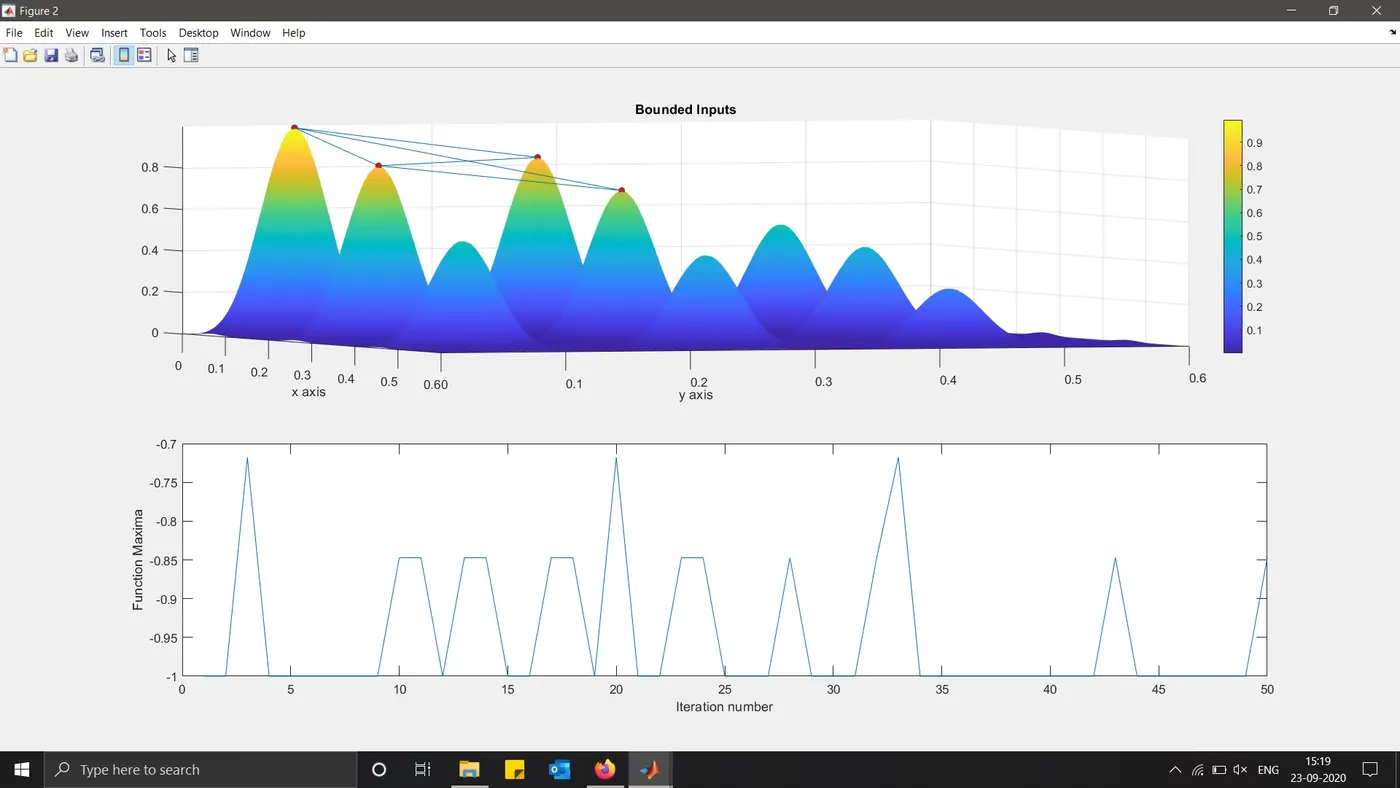
Here in this case, in the coding everything remains the same except of the GA syntax used is “x = ga(fun,nvars,A,b)” therefore in the “for loop” the following command was written “[inputs, fopt(k)] = ga(@stalagmite_func, 2, [],[],[],[],[0 0],[1 1])”. Where we are bounding the input values of the input vector “X” and “Y” upper and lower limits [0 0] and [1 1], which gives us a refined plots of “xopt”, “yopt” and “fopt”. Unlike the first case where we had the plot of multiple points scattered in the plot space, here in this case we just have four points plotted, which are predicted by the GA function that minimum point is between the four points of the peaks as shown in the figure in the results section.

Programming for Case 3, increasing number of iterations:

num_cases = 50;
tic
% Increasing the GA population to pick the number of optimization, where
% more population means better result: Case 3

options = optimoptions('ga');
options = optimoptions(options,'PopulationSize',350);

for l = 1:num_cases
    [inputs, fopt(l)] = ga(@stalagmite_func, 2, [],[],[],[],[0 0],[1 1],[],[],options);
    xopt(l) = inputs(1);
    yopt(l) = inputs(2);
end
case_time_Case3 = toc

figure(3)
subplot(2,1,1)
surfc(xx,yy,-f)
xlabel('x values')
ylabel('y values')
shading interp
colorbar
hold on
plot3(xopt,yopt,-fopt,'marker','o','markersize',5,'markerfacecolor','k')
title('Optimization with large population')
xlabel('x axis')
ylabel('y axis')   

subplot(2,1,2)
plot(fopt)
xlabel('Iteration number')
ylabel('Function Maxima')

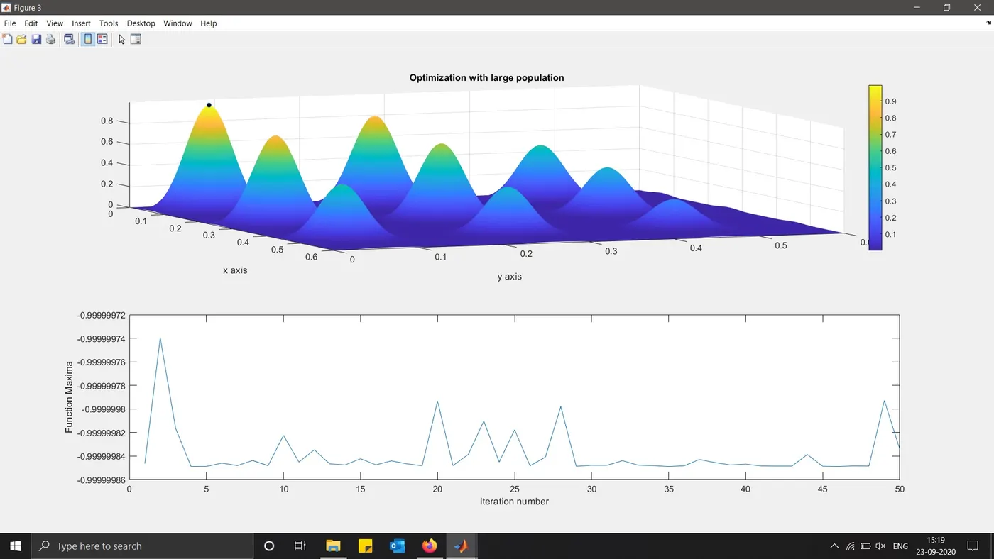
Here in this case, the GA syntax for the calculations used was, “x = ga(fun,nvars,A,b,Aeq,beq,lb,ub,nonlcon,options)” where we have an input called “options” which is nothing but the “Population Size” that is number of iterations (350) are considered for GA calculations. By doing this we get much refined graph where we have one point plotted in the graph which gives us the function maxima predicted by the GA. Here we plotted “fopt” which is predicted by GA along with “xopt” and “yopt”. The plot can be seen in the results section of this project.

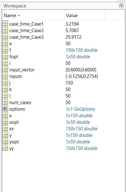
The case running time that the algorithm took to run is shown in the figure below along with the other values such as inputs, input vectors, and the values of e, k, l can be seen in the figure.

Results:

The plots of the GA predictions for Case 1, Case 2 and Case 3 are shown in the figures below.

Plot of Case 1

Plot of Case 2

Plot of Case 3

Conclusions:

1. The plots were made successfully for all three cases
2. A couple of errors were faced during executing the first and third cases. Where in the first case, there was a mistake made in writing the “shading interp” command where there was no space given between two words, which was rectified later. Thereafter in Case 3 there was a mistake made in writing “optimoptions” where it was written “optoptions” which was then rectified by using Matlab help.

References:

[1] https://www.pico.net/kb/how-does-a-genetic-algorithm-work

[2] https://in.mathworks.com/help/gads/how-the-genetic-algorithm-works.html

[3] https://in.mathworks.com/help/gads/ga.html