Curve Fitting: Fitting curves using linear curve, quadratic curve, cubic curve and split-wise curve fitting methods.
Aim:
- To write a code to plot and fit linear and cubic polynomial for the Cp data.
- To write a code to show and plot the split-wise method to fit the curve and compare the raw data and the fitted curve.
- To calculate the errors in the curve and to determine the perfect and the best fit of the curves.
Description:
Curve fitting is one of the most widely used analysis methods to construct a curve or math functions that possess the close proximity to the original data series. Curve fitting method examines the relationship between one or more predictors and a response variable, with the goal of defining a "best fit" or “perfect fit” model of the relationship which can be determined by calculating R2 error. In curve fitting the functional relationship can be mathematically constructed between observed dataset (original dataset) and the parameter values.
In curve fitting we can fit curves using the linear regression method, which is the most common method. In this method we can include the polynomial terms in the linear models. Polynomial terms are independent variables in which we can raise to a power, for instance to the power of square or cube.
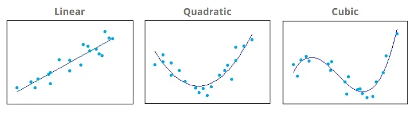
The three most common types are as shown in the figure below:
Most commonly the curve is fitted by the function y=f(x). Here the first degree of polynomial equation can be considered as:
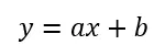
which connects generally two points in the curve as a slope.
If the degree of the order is increased to the second degree polynomial the polynomial equation can be considered as:
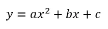
This equation will exactly fit a curve to three points. If the order of degree is increased to third degree the equation will be:

This equation will exactly fit a curve to four points. These equations will form a linear, a quadratic and a cubic curve, respectively.
There are four parameters used to choose a best fit which are:
- Sum of squares due to errors (SSE)
- R square
- Adjusted R square
- Root mean squared error.
To fit a curve perfectly, we need to increase the degree of polynomial or use the split-wise curve fitting method. As discussed ahead in this project, it is shown how a curve was fitted using a higher degree polynomial. Thereafter split-wise method to fit the curve was executed where the curve was a perfect fit.
Theory:
% Curve Fitting using Matlab

clear all
close all
clc

% To prepare the data
cp_data = load('data');
temperature = cp_data(:,1);
cp = cp_data(:,2);

% Curve Fitting
% 1 degree linear polinomial, cp = a*T + C

co_effs = polyfit(temperature,cp,1);
predicted_cp = polyval(co_effs,temperature);

% Compare curvefit with original data

figure(1)
hold on
plot(temperature,cp,'linewidth',3,'color','k')
plot(temperature,predicted_cp,'linewidth',3,'color','r')
xlabel('Temperature[K]')
ylabel('Specific heat[KJ/Kmo-K]')
title('Linear Curve Fit')
legend('original dataset','curvefit','location','northwest')

% Calculating error using R^2 method for linear polinomial

mean = sum(cp)/length(cp);
ssr = (predicted_cp - mean).^2;
sse = (cp - predicted_cp).^2;

SSR = sum(ssr);
SSE = sum(sse);
R2_1 = SSR/(SSR+SSE)


% 2 degree quadratic polinomial, cp = a*T^2+b*T+C

co_effs = polyfit(temperature,cp,2);
predicted_cp = polyval(co_effs,temperature);

% Compare curvefit with original data

figure(2)
hold on
plot(temperature,cp,'linewidth',3,'color','k')
plot(temperature,predicted_cp,'linewidth',3,'color','r')
xlabel('Temperature[K]')
ylabel('Specific heat[KJ/Kmo-K]')
title('Quadratic Curve Fit')
legend('original dataset','curvefit','location','northwest')

% Calculating error using R^2 method for quadratic polinomial

mean = sum(cp)/length(cp);
ssr = (predicted_cp - mean).^2;
sse = (cp - predicted_cp).^2;

SSR = sum(ssr);
SSE = sum(sse);
R2_2 = SSR/(SSR+SSE)


% 3 degree cubic polinomial, cp = a*T^3 + b*T^2 + c*T + C

co_effs = polyfit(temperature,cp,3);
predicted_cp = polyval(co_effs,temperature);

% Compare curvefit with original data

figure(3)
hold on
plot(temperature,cp,'linewidth',3,'color','k')
plot(temperature,predicted_cp,'linewidth',3,'color','r')
xlabel('Temperature[K]')
ylabel('Specific heat[KJ/Kmo-K]')
title('Cubic Curve Fit')
legend('original dataset','curvefit','location','northwest')

% Calculating error using R^2 method for cubic polinomial

mean = sum(cp)/length(cp);
ssr = (predicted_cp - mean).^2;
sse = (cp - predicted_cp).^2;

SSR = sum(ssr);
SSE = sum(sse);
R2_3 = SSR/(SSR+SSE)
% Split-wise curve fitting using Matlab
clear all
close all
clc
% To prepare the data
cp_data = load('data');
temperature = cp_data(:,1);
cp = cp_data(:,2);
% Splitting the curve in 6 parts, dividing the data of temperature and cp
% into four parts of 3200 i.e. 500, 1000, 1500, 2000, 2500, 3200
% Calculating the curve for split 1 (1-500)
% cp and temperature values
temperature_1 = cp_data(1:500,1);
cp_1 = cp_data(1:500,2);
% coefficients and predicted cp for curve 1
[co_eff_1, S1, mu1] = polyfit(temperature_1, cp_1, 3);
predicted_cp_1 = polyval(co_eff_1, temperature_1,[],mu1);
% Calculating the curve for split 2 (501-1000)
% cp and temperature values
temperature_2 = cp_data(501:1000,1);
cp_2 = cp_data(501:1000,2);
% coefficients and predicted cp for curve 2
[co_eff_2, S2, mu2] = polyfit(temperature_2, cp_2, 3);
predicted_cp_2 = polyval(co_eff_2, temperature_2,[],mu2);
% Calculating the curve for split 3 (1001-1500)
% cp and temperature values
temperature_3 = cp_data(1001:1500,1);
cp_3 = cp_data(1001:1500,2);
% coefficients and predicted cp for curve 3
[co_eff_3, S3, mu3] = polyfit(temperature_3, cp_3, 3);
predicted_cp_3 = polyval(co_eff_3, temperature_3,[],mu3);
% Calculating the curve for split 4 (1501-2000)
% cp and temperature values
temperature_4 = cp_data(1501:2000,1);
cp_4 = cp_data(1501:2000,2);
% coefficients and predicted cp for curve 4
[co_eff_4, S4, mu4] = polyfit(temperature_4, cp_4, 3);
predicted_cp_4 = polyval(co_eff_4, temperature_4,[],mu4);
% Calculating the curve for split 5 (2001-2500)
% cp and temperature values
temperature_5 = cp_data(2001:2500,1);
cp_5 = cp_data(2001:2500,2);
% coefficients and predicted cp for curve 5
co_eff_5 = polyfit(temperature_5, cp_5, 2);
predicted_cp_5 = polyval(co_eff_5, temperature_5);
% Calculating the curve for split 6 (2501-3200)
% cp and temperature values
temperature_6 = cp_data(2501:3200,1);
cp_6 = cp_data(2501:3200,2);
% coefficients and predicted cp for curve 6
co_eff_6 = polyfit(temperature_6, cp_6, 2);
predicted_cp_6 = polyval(co_eff_6, temperature_6);
% Predicted_cp vector for error calculation
predicted_cp = [predicted_cp_1;predicted_cp_2;predicted_cp_3;predicted_cp_4;predicted_cp_5;predicted_cp_6];
% Comparing original curve with curve fit
% Original data curve
plot(temperature,cp,'linewidth',5,'color','r')
hold on
% Split Curve fit
plot(temperature_1, predicted_cp_1, 'linewidth', 2, 'color', 'y')
plot(temperature_2, predicted_cp_2, 'linewidth', 2, 'color', 'b')
plot(temperature_3, predicted_cp_3, 'linewidth', 2, 'color', 'g')
plot(temperature_4, predicted_cp_4, 'linewidth', 2, 'color', 'k')
plot(temperature_5, predicted_cp_5, 'linewidth', 2, 'color', 'm')
plot(temperature_6, predicted_cp_6, 'linewidth', 2, 'color', 'w')
xlabel('Temperature[K]')
ylabel('Specific heat[KJ/Kmo-K]')
legend('original dataset','curve1','curve2','curve3','curve4','curve5','curve6','location','northwest')
title('Splitwise Curvefit')
% Error Calculation, calculating R^2 value
mean = sum(cp)/length(cp);
ssr = (predicted_cp - mean).^2;
sse = (cp-predicted_cp).^2;
SSR = sum(ssr);
SSE = sum(sse);
R_square = SSR/(SSR+SSE)Explaination for normal linear, quadratic and cubic curve fitting:
In the first case linear, quadratic, and cubic curves were fitted along the raw data set. Where the following commands were written to plot and fit the curves.
% Curve Fitting using Matlab
clear all
close all
clc
% To prepare the data
cp_data = load('data');
temperature = cp_data(:,1);
cp = cp_data(:,2);Normal “clear all”, “close all”, and “clc” were written to close any running program and to clear any data in the workspace and to clear any text or outputs in the command window. Thereafter the command to extract the raw data of temperature and cp was extracted using the “load” command where “cp_data = load(‘data’)” was written to bring the already provided data file into the Matlab software, where that data can be calculated and plotted respectively. Thereafter, temperature and cp data was extracted individually and assigned to its respective parameters such as “temperature = cp_data(:,1)” was written as the first column of the data was the temperature values in kelvin. And then cp values were extracted using “cp = cp_data(:,2)” where second column in the dataset was the cp values.
Thereafter, a first degree linear curve fit was executed as well as calculating the R2 value to determine the type of fit of the curve using the following commands:
% Curve Fitting
% 1 degree linear polinomial, cp = a*T + C
co_effs = polyfit(temperature,cp,1);
predicted_cp = polyval(co_effs,temperature);
% Compare curvefit with original data
figure(1)
hold on
plot(temperature,cp,'linewidth',3,'color','k')
plot(temperature,predicted_cp,'linewidth',3,'color','r')
xlabel('Temperature[K]')
ylabel('Specific heat[KJ/Kmo-K]')
title('Linear Curve Fit')
legend('original dataset','curvefit','location','northwest')
% Calculating error using R^2 method for linear polinomial
mean = sum(cp)/length(cp);
ssr = (predicted_cp - mean).^2;
sse = (cp - predicted_cp).^2;
SSR = sum(ssr);
SSE = sum(sse);
R2_1 = SSR/(SSR+SSE)The 1st degree linear polynomial was plotted using the above command. Where, “polyfit” command was used to calculate the values of the coefficients of the polynomials that best fits the data, allocated to the term “co_effs” that are the coefficients of the polynomial. The command written was “co_effs= polyfit(temperature, cp, 1)”. Here in this command the temperature and cp values were inserted along the degree of the polynomial which was “1” for linear curve fit. Thereafter the new cps were predicted by allocating the term ”predicted_cp” where “polyval” command was used to calculate the value of polynomial where the previously calculated coefficients along with the temperature were inserted as “predicted_cp = polyval(co_effs, temperature)” here the co_effs is the vector with the coefficients of the polynomial and temperature is the number or a variable that has an assigned value to it.
Thereafter, the curve was plotted against the raw dataset that is temperature vs cp and the plot of temperature vs predicted_cp was plotted in the same plot to compare the fit.
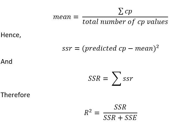
The curve fit error R2 was then calculated by calculating SSE and SSR, where, SSE is:

And SSE is the sum of all the values of sse.
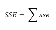
SSR was calculated by first calculating the mean of all the cp values, the mean was calculated by using the following formula in Matlab.
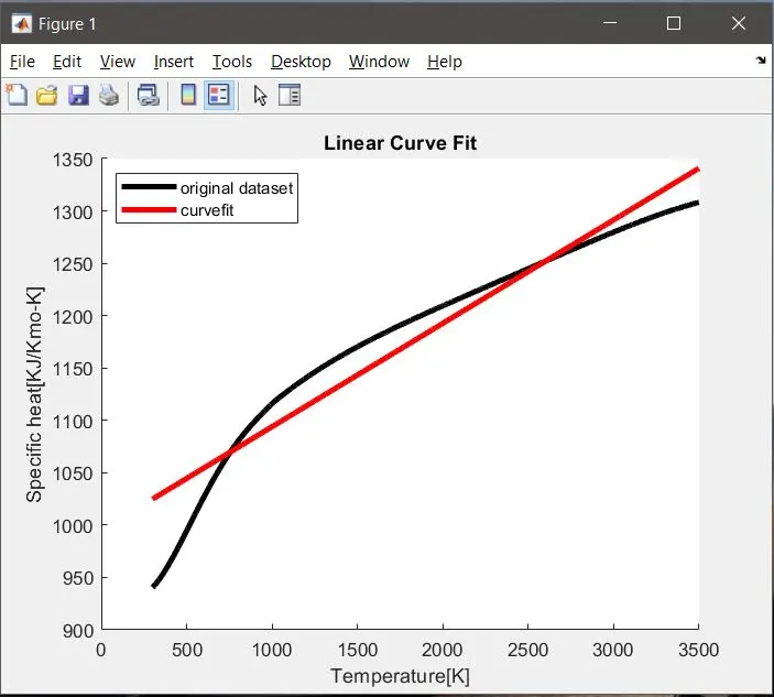
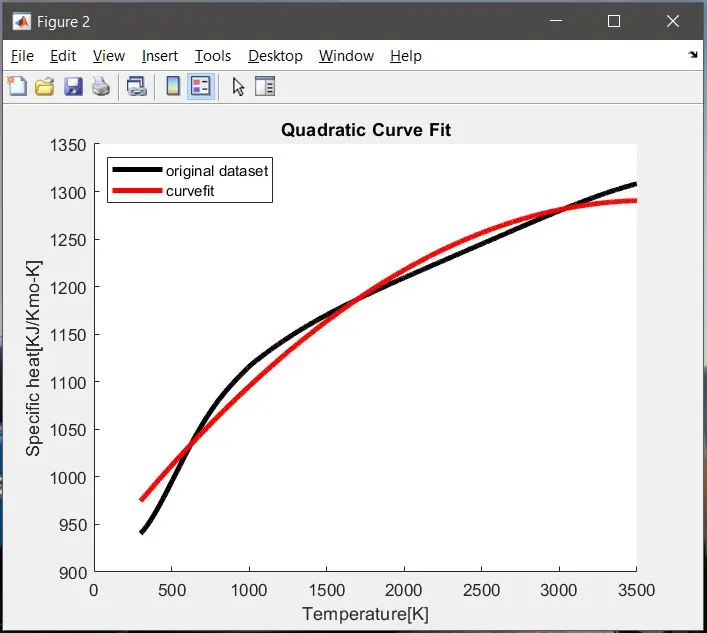
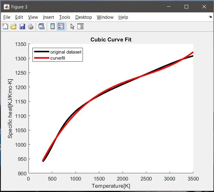
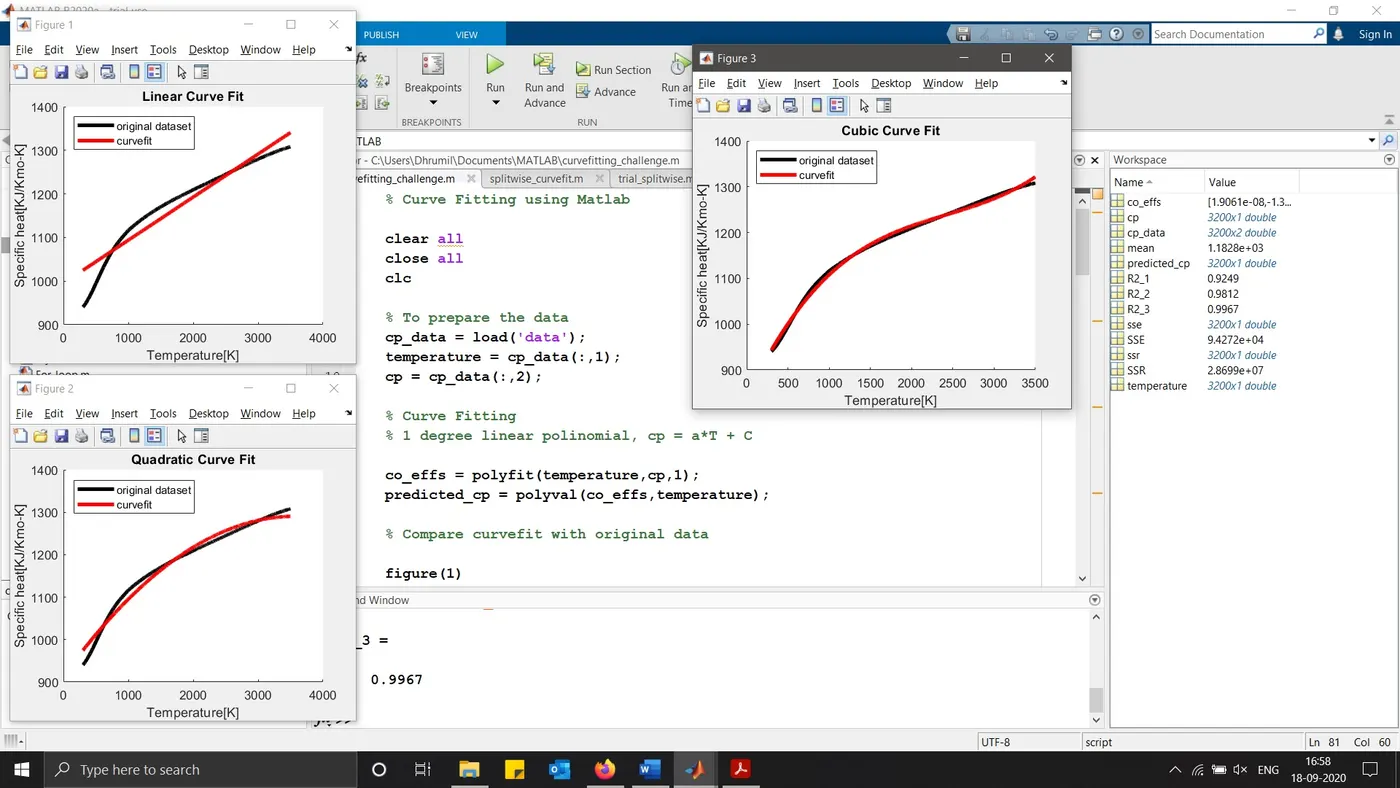
The same commands were used to calculate the quadratic and the cubic curves where the only difference was that the degree of polynomial was changed to “2” and “3” respectively. The final plots of linear, quadratic and cubic curves are represented as below in the results section, and the values of R2 for all three cases are as below:
R2 for linear curve obtained was 0.9249
R2 for quadratic curve obtained was 0.9812 and
R2 for cubic curve obtained was 0.9967.
However, after executing the whole program, a warning was observed in the command window saying that “Polynomial is badly conditioned. Add points with distinct X values, reduce the degree of the polynomial”.
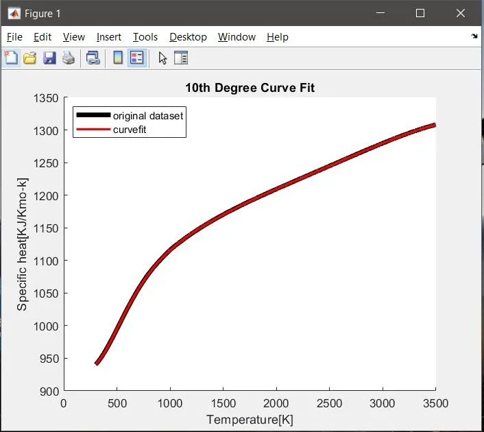
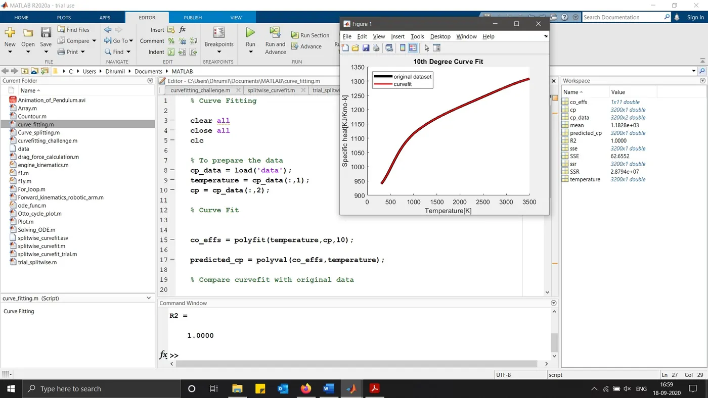
It was observed that when the degree of the polynomial was increased, the curve was fitting smoothly and hence getting the best fit of the curve. The best fit of the curve is determined by the R2 error values which lies between 0 to 1 where 1 being the perfect fit. Here we can say that by using 1, 2 and 3 degree of polynomials we can get the best fit however, if the degree was changed to 10 a perfect fit was achieved as shown in the figure below (in the results section) with the R2 value being 1, however, the warning still remained that the polynomial was badly conditioned. Therefore it can be said that the best fit can be achieved by using higher degree polynomial. Hence the split-wise curve fitting was executed as discussed further on.
To improve the cubic fit the command [p,S,mu] = polyfit(x,y,n] can be used where “mu” is the two element vector with centring and scaling values, “p” is the coefficient, S is the structure, mu(1) is the mean and mu(2) is the standard deviation. Using these values “polyfit” command centres x at 0 and scales it to have a standard deviation [1]. This is used further in the split-wise curve fit method to improve the 4 cubic curves out of 6, where the remaining two curves were quadratic as the bend in the curve did not need any conditioning. As tried before using all the split-wise curves as 2nd degree quadratic curves, the starting curves were not smooth (as shown in the figure in the end of the project), then by trial and error method the first four curves were made cubic curves with more improvements using [p,s,mu] command in Matlab, thereafter the initial curves were found to be smooth.
Explaination for Split-wise Curve Fit:
% Split-wise curve fitting using Matlab

clear all
close all
clc

% To prepare the data
cp_data = load('data');
temperature = cp_data(:,1);
cp = cp_data(:,2);


% Splitting the curve in 6 parts, dividing the data of temperature and cp
% into four parts of 3200 i.e. 500, 1000, 1500, 2000, 2500, 3200

% Calculating the curve for split 1 (1-500)
% cp and temperature values
temperature_1 = cp_data(1:500,1);
cp_1 = cp_data(1:500,2);

% coefficients and predicted cp for curve 1
[co_eff_1, S1, mu1] = polyfit(temperature_1, cp_1, 3);
predicted_cp_1 = polyval(co_eff_1, temperature_1,[],mu1);


% Calculating the curve for split 2 (501-1000)
% cp and temperature values
temperature_2 = cp_data(501:1000,1);
cp_2 = cp_data(501:1000,2);

% coefficients and predicted cp for curve 2
[co_eff_2, S2, mu2] = polyfit(temperature_2, cp_2, 3);
predicted_cp_2 = polyval(co_eff_2, temperature_2,[],mu2);


% Calculating the curve for split 3 (1001-1500)
% cp and temperature values
temperature_3 = cp_data(1001:1500,1);
cp_3 = cp_data(1001:1500,2);

% coefficients and predicted cp for curve 3
[co_eff_3, S3, mu3] = polyfit(temperature_3, cp_3, 3);
predicted_cp_3 = polyval(co_eff_3, temperature_3,[],mu3);


% Calculating the curve for split 4 (1501-2000)
% cp and temperature values
temperature_4 = cp_data(1501:2000,1);
cp_4 = cp_data(1501:2000,2);

% coefficients and predicted cp for curve 4
[co_eff_4, S4, mu4] = polyfit(temperature_4, cp_4, 3);
predicted_cp_4 = polyval(co_eff_4, temperature_4,[],mu4);


% Calculating the curve for split 5 (2001-2500)
% cp and temperature values
temperature_5 = cp_data(2001:2500,1);
cp_5 = cp_data(2001:2500,2);

% coefficients and predicted cp for curve 5
co_eff_5 = polyfit(temperature_5, cp_5, 2);
predicted_cp_5 = polyval(co_eff_5, temperature_5);


% Calculating the curve for split 6 (2501-3200)
% cp and temperature values
temperature_6 = cp_data(2501:3200,1);
cp_6 = cp_data(2501:3200,2);

% coefficients and predicted cp for curve 6
co_eff_6 = polyfit(temperature_6, cp_6, 2);
predicted_cp_6 = polyval(co_eff_6, temperature_6);


% Predicted_cp vector for error calculation
predicted_cp = [predicted_cp_1;predicted_cp_2;predicted_cp_3;predicted_cp_4;predicted_cp_5;predicted_cp_6];


% Comparing original curve with curve fit
% Original data curve

plot(temperature,cp,'linewidth',5,'color','r')
hold on

% Split Curve fit
plot(temperature_1, predicted_cp_1, 'linewidth', 2, 'color', 'y')
plot(temperature_2, predicted_cp_2, 'linewidth', 2, 'color', 'b')
plot(temperature_3, predicted_cp_3, 'linewidth', 2, 'color', 'g')
plot(temperature_4, predicted_cp_4, 'linewidth', 2, 'color', 'k')
plot(temperature_5, predicted_cp_5, 'linewidth', 2, 'color', 'm')
plot(temperature_6, predicted_cp_6, 'linewidth', 2, 'color', 'w')


xlabel('Temperature[K]')
ylabel('Specific heat[KJ/Kmo-K]')
legend('original dataset','curve1','curve2','curve3','curve4','curve5','curve6','location','northwest')
title('Splitwise Curvefit')

% Error Calculation, calculating R^2 value
mean = sum(cp)/length(cp);
ssr = (predicted_cp - mean).^2;
sse = (cp-predicted_cp).^2;

SSR = sum(ssr);
SSE = sum(sse);

R_square = SSR/(SSR+SSE)For split-wise method the curve was divided into 6 parts. Where the number of dataset containing rows was 3200 and it was divided into 500 number of dataset for each curve where the last curve consisted of 700 rows of data which is optimal. Therefore, for the first curve 1-500 rows of data, for second curve 501-1000, for third 1001-1500, for fourth 1501-2000, for fifth 2001-2500 and for sixth 2501-3200 dataset rows were considered for calculations.
% Split-wise curve fitting using Matlab

clear all
close all
clc

% To prepare the data
cp_data = load('data');
temperature = cp_data(:,1);
cp = cp_data(:,2);
Starting to write the codes, clear all, close all, clc were written for closure of programs and clearing the screens. Thereafter, the data was extracted from the prior given dataset file. The data extraction commands were used as explained previously in the curve fitting commands.
Thereafter the calculation commands were written for each of the six curves as shown below:
% Splitting the curve in 6 parts, dividing the data of temperature and cp
% into four parts of 3200 i.e. 500, 1000, 1500, 2000, 2500, 3200

% Calculating the curve for split 1 (1-500)
% cp and temperature values
temperature_1 = cp_data(1:500,1);
cp_1 = cp_data(1:500,2);

% coefficients and predicted cp for curve 1
[co_eff_1, S1, mu1] = polyfit(temperature_1, cp_1, 3);
predicted_cp_1 = polyval(co_eff_1, temperature_1,[],mu1);


% Calculating the curve for split 2 (501-1000)
% cp and temperature values
temperature_2 = cp_data(501:1000,1);
cp_2 = cp_data(501:1000,2);

% coefficients and predicted cp for curve 2
[co_eff_2, S2, mu2] = polyfit(temperature_2, cp_2, 3);
predicted_cp_2 = polyval(co_eff_2, temperature_2,[],mu2);


% Calculating the curve for split 3 (1001-1500)
% cp and temperature values
temperature_3 = cp_data(1001:1500,1);
cp_3 = cp_data(1001:1500,2);

% coefficients and predicted cp for curve 3
[co_eff_3, S3, mu3] = polyfit(temperature_3, cp_3, 3);
predicted_cp_3 = polyval(co_eff_3, temperature_3,[],mu3);


% Calculating the curve for split 4 (1501-2000)
% cp and temperature values
temperature_4 = cp_data(1501:2000,1);
cp_4 = cp_data(1501:2000,2);

% coefficients and predicted cp for curve 4
[co_eff_4, S4, mu4] = polyfit(temperature_4, cp_4, 3);
predicted_cp_4 = polyval(co_eff_4, temperature_4,[],mu4);
Here for the first four curves the cubic curves were implemented and as explained above the [p,S,mu] commands were used for each of the first four curves, where the coefficients of the polynomials and the predicted cps were calculated. “[co_eff_1, S1, mu1] = polyfit(temperature_1, cp_1, 3)” was used to calculate the coefficients for the first curve hence “[co_eff_1, S1, mu1]” was written including “1” to indicate that these are for the curve one and so on as “2”, “3”, “4” for other four curves.
% Calculating the curve for split 5 (2001-2500)
% cp and temperature values
temperature_5 = cp_data(2001:2500,1);
cp_5 = cp_data(2001:2500,2);

% coefficients and predicted cp for curve 5
co_eff_5 = polyfit(temperature_5, cp_5, 2);
predicted_cp_5 = polyval(co_eff_5, temperature_5);


% Calculating the curve for split 6 (2501-3200)
% cp and temperature values
temperature_6 = cp_data(2501:3200,1);
cp_6 = cp_data(2501:3200,2);

% coefficients and predicted cp for curve 6
co_eff_6 = polyfit(temperature_6, cp_6, 2);
predicted_cp_6 = polyval(co_eff_6, temperature_6);
The above shown command was written for the fifth and sixth curves indicating “5” and “6” in the commands, the fifth and sixth curves were of 2nd degree polynomial therefore “2” is given as an input in the “polyfit” command. Thereafter the pridected_cp were calculated for both of the split curves.
% Predicted_cp vector for error calculation
predicted_cp = [predicted_cp_1;predicted_cp_2;predicted_cp_3;predicted_cp_4;predicted_cp_5;predicted_cp_6];
After calculating predicted_cp_1, predicted_cp_2, predicted_cp_3, predicted_cp_4, predicted_cp_5, predicted_cp_6 for all six curves, they were formed to be a vector quantity, to bring them under one entity that is “predicted_cp”
% Comparing original curve with curve fit
% Original data curve

plot(temperature,cp,'linewidth',5,'color','r')
hold on

% Split Curve fit
plot(temperature_1, predicted_cp_1, 'linewidth', 2, 'color', 'y')
plot(temperature_2, predicted_cp_2, 'linewidth', 2, 'color', 'b')
plot(temperature_3, predicted_cp_3, 'linewidth', 2, 'color', 'g')
plot(temperature_4, predicted_cp_4, 'linewidth', 2, 'color', 'k')
plot(temperature_5, predicted_cp_5, 'linewidth', 2, 'color', 'm')
plot(temperature_6, predicted_cp_6, 'linewidth', 2, 'color', 'w')
To compare the raw data and the split curves data, which is calculated above, the curve plots were made. Plotting the raw data temperature vs cp first, thereafter using “hold on” command to plot the six curves into the same window in order to compare our split curve fit. Therefore, the above commands were written to original curve and the six split curves. Here the original curve was given a “linewidth” of “5” and the split curves width was given as “2” for presentation purpose so the original curve is visible with the split curves. Thereafter all split curves were given different colours, so all the six curves are visible distinctively. In the end the x-axis, y-axis labels the title of the plot and the legend for the plots were defined as shown below.
xlabel('Temperature[K]')
ylabel('Specific heat[KJ/Kmo-K]')
legend('original dataset','curve1','curve2','curve3','curve4','curve5','curve6','location','northwest')
title('Splitwise Curvefit')
Thereafter to calculate the R2 error for the split fitted curve was calculated using the below described command.
% Error Calculation, calculating R^2 value
mean = sum(cp)/length(cp);
ssr = (predicted_cp - mean).^2;
sse = (cp-predicted_cp).^2;

SSR = sum(ssr);
SSE = sum(sse);

R_square = SSR/(SSR+SSE)
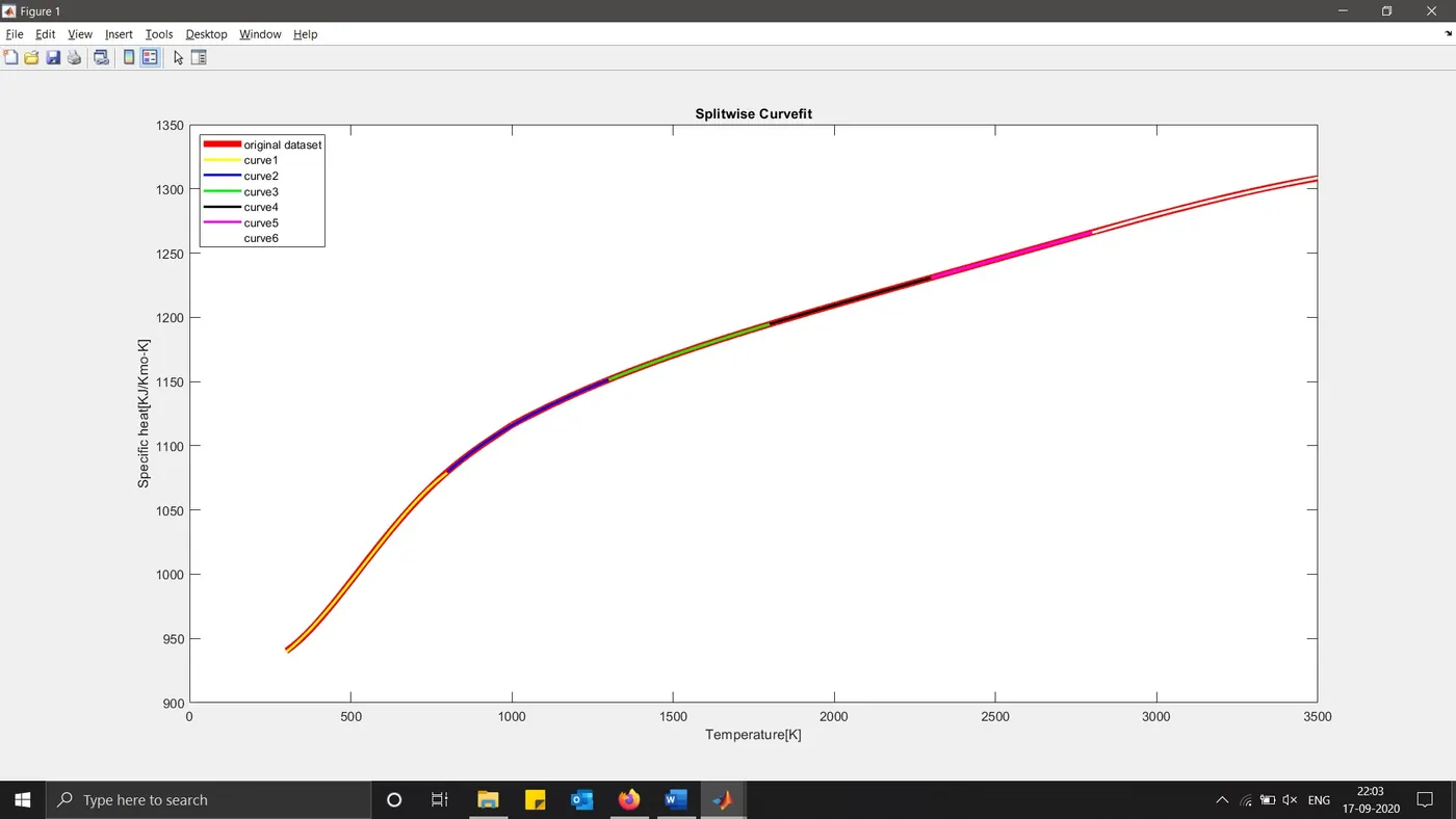
Here the “predicted_cp” is inserted which is one vector of all the “predicted_cp” values of all six curves. Where SSR and SSE are calculated for the calculation of R2. The R2 here was observed to be 1, which is “Perfect Fit”. The plot of the split-wise curve fitting is as shown below in the results section.
Results:
- The R2 values for the linear, quadratic, and cubic curves were observed as best fit and the values of R2 of all three curves are 0.9249, 0.9812 and 0.9967 and the plots are as shown below.
- The split-wise curve fitting was executed and the R2 was observed to be 1 which is perfect fit and the plot is as shown below.
Linear Curve Fit
Quadratic Curve Fit
Cubic Curve Fit
10th Degree Curve Fit
Split-wise Curve Fit
Conclusion:
- It was observed that, by increasing the polynomial degree of the polynomial the curve was made to fit perfectly.
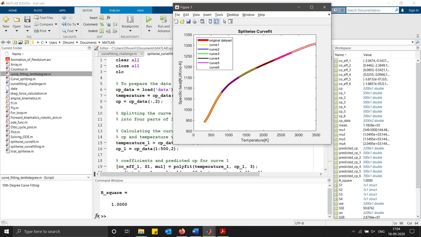
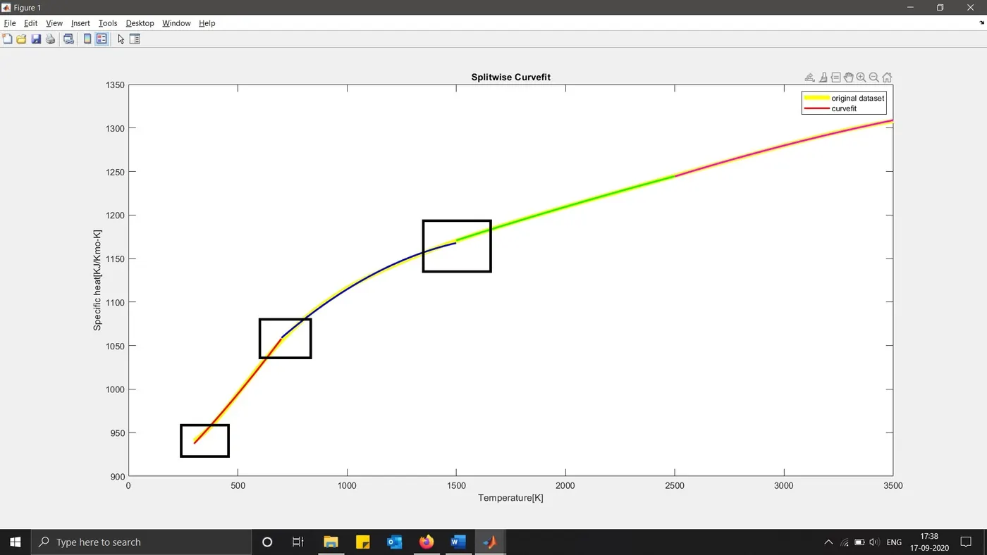
- It was observed, by using the 1st or 2nd degree polynomial for the initial curves in split-wise curve fitting, the curves were not smooth, however by trial and error and by using 3rd degree polynomial and by using [p,S,mu] in 3rd degree polynomial the curves were made smoother.
- Initially for the split-wise curve fitting, the curve fit was split into four parts and then later, the curve was split into six parts, this was a part of trial and error to see how much of a difference occurs while plotting, however there was no as such difference observed, but the curve fit plotted was smooth, and in the end the six curve split-wise curve fitting was considered for the project.
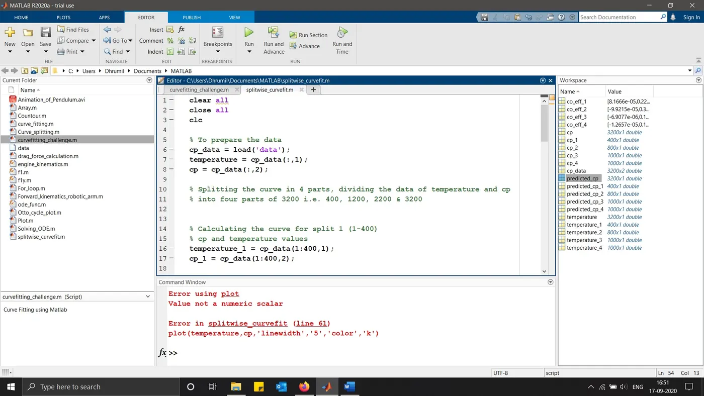
- There was one error that was faced once while plotting the split-wise curves as shown below, which was nothing but the error of the “linewidth” value which was inserted in “5” where “” are not used to input the “linewidth” value only numeric value is inserted.
The screenshots of the Matlab window are as below, including the asymmetric initial curves in the split-wise curve fitting.
Error in Split-wise program
10th Degree Curve Fit
References: