BAJA ATV System Level Simulation and Analysis

Aim:

1. To simulate the BAJA ATV model by MathWorks.
2. To explain the vehicle parameters.
3. To discuss the final results.

Objectives:

1. To simulate the ATV model with and without dashboard.
2. To simulate the ATV model with and without dashboard having Lookup table.

Theory:

BAJA: BAJA is an inter college competition which is conducted by SAE whose main focus is the outside classroom education in automotive engineering. This competition focuses on racing of All Terrain Vehicles (ATVs) which are built by undergraduate or graduate level engineering students. Each year as many as 141 Baja cars are entered in the Baja SAE events across the US and around the world where events are endorsed by SAE International [1][2].

ATV: All Terrain Vehicles refer to the single seater motorised vehicle which can run on every type of terrain be it on road or off-road. These vehicles have low pressure deep threaded tires which can handle rocky or muddy terrain. These vehicles can also be customised for high performance racing, for different agricultural utilities, industrial applications as a carrier or for defence purposes. These vehicles have a rigid structure, enabling rider safety as it is an off-road vehicle.

CVT: CVT refers to continuous variable transmission, which is an automatic transmission with single speed. This transmission can shift various gear ratios. The flexibility of a CVT with suitable control may allow the engine to operate at a constant RPM while the vehicle moves at varying speeds. CVTs are used in various types of vehicles such as cars, tractors, snow mobiles, moped scooters, and ATVs [3].

Part 1: BAJA ATV Simulink Models without Lookup table.

Part 1.1: ATV Model without Dashboard.

The Simulink model of ATV with no dashboard can be seen below.

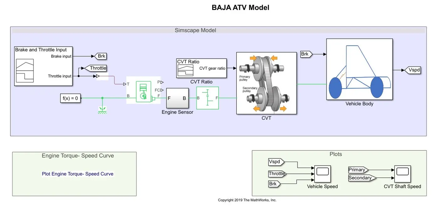
As seen above the throttle and brake inputs are given by the Signal builder block of Simulink. Where two output of throttle is given to the Generic engine block, which represents as the engine of the vehicle in the model. The linear signals are given to run the model according to the functioning required in the model. The input signal from the signal builder can be seen in the figure below.

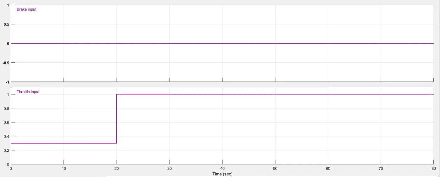
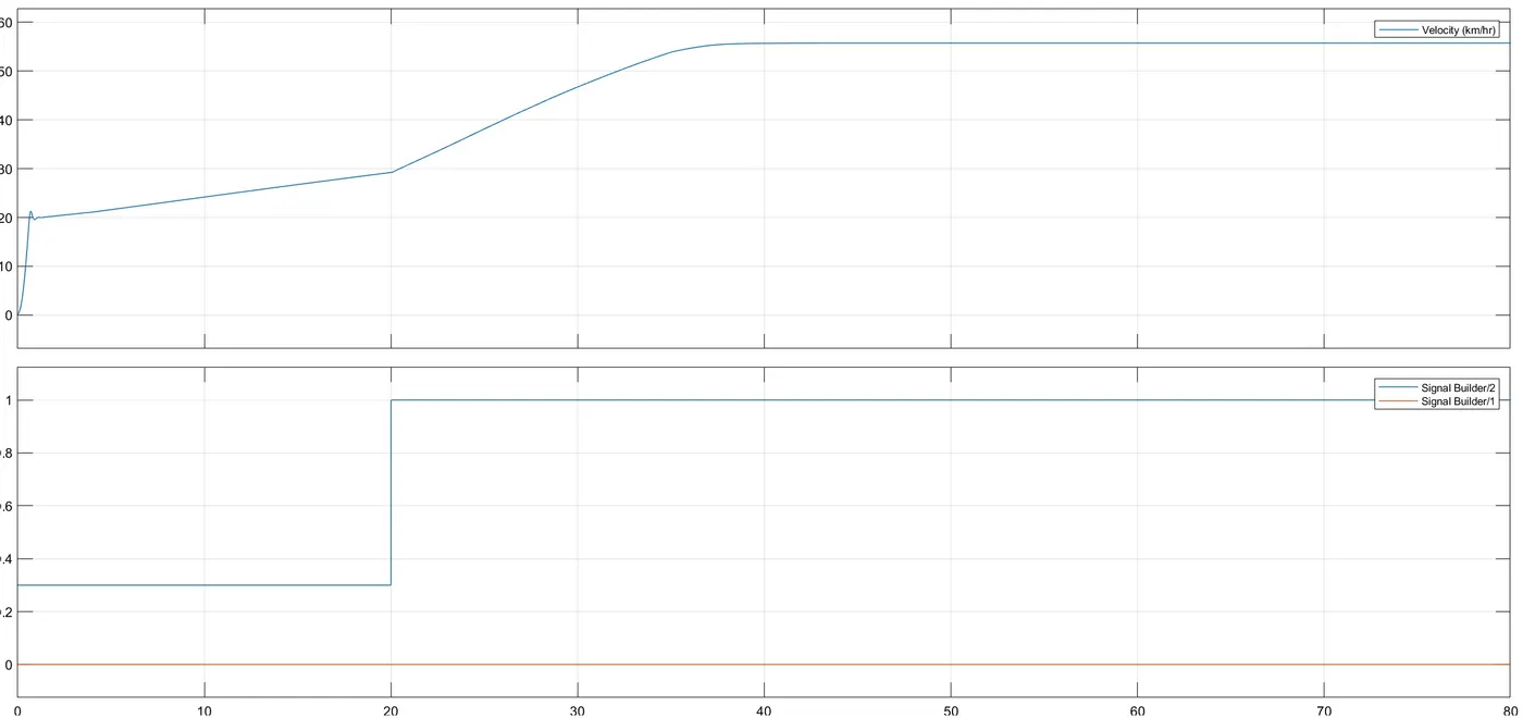
Here it can be seen that the brake input signal line is set to zero and the throttle is set for 0.3 for first 20 seconds and at 1 for rest 60 seconds totalling 80 seconds of one cycle.

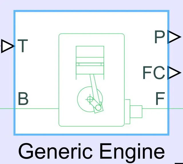
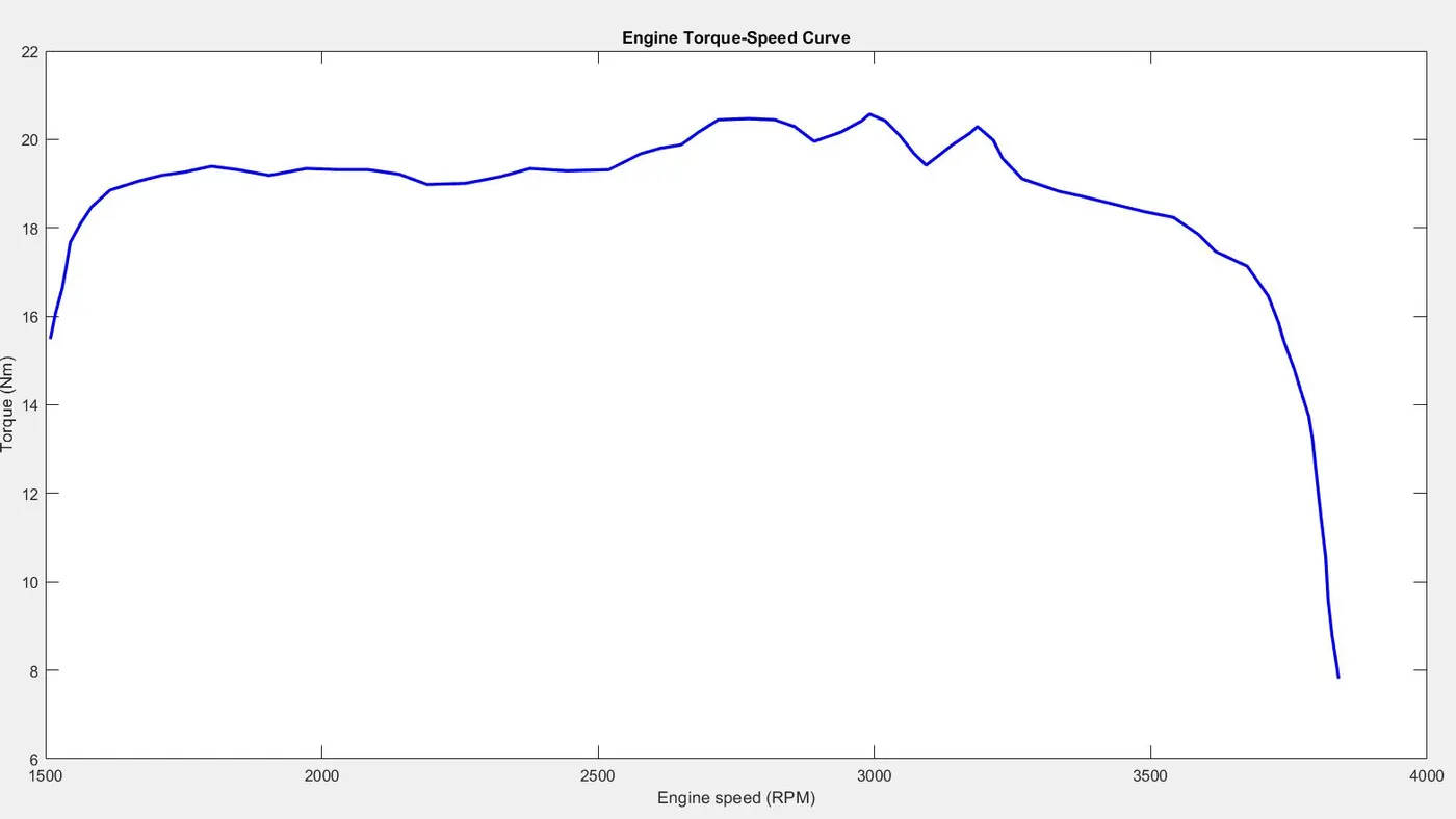
The signal from the signal builder block was then given to the port T of the generic engine block which is the throttle input of the engine. The ports B and F are the mechanical rotational conserving ports associated with the engine crankshaft and engine block. The out put was then given to the engine sensor via F port. This engine was configured with “speed vector” and “torque vector” which are real time data from the actual vehicle, which was input externally from the Matlab, which can be seen in the figure below.

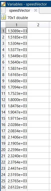
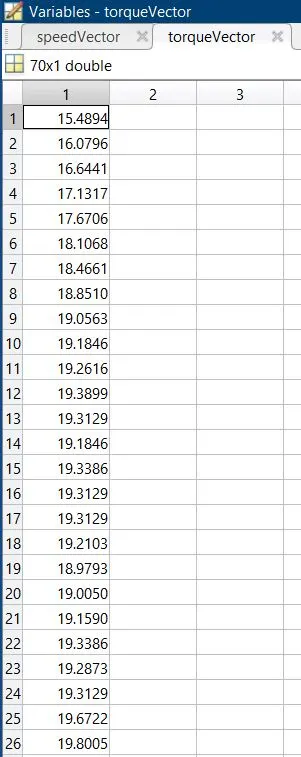
For engine block parameters, the settings were made by default to capture the data from these two tables and the speed vector was given the unit as rpm and the torque vector as N*m. The B port of the engine was connected to a rotational reference and was connected to a solver configuration for whole system. The F port connected to the engine sensor, the engine sensor block can be seen below, which is built with the RPM sensor to sense the RPM of the engine from the output shaft of the engine.

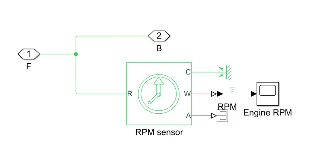
Here from the rpm sensor the output goes to a “simple gear” block which is connected to the CVT transmission block. The engine sensor is basically is to detect the engine rpm which can be seen through the scope attached to the sensor. The C port is connected to the rotational reference for the block. Here in this block, the F port is the input port and B is the output port, where B is connected to a simple gear block as shown below.

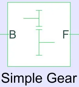
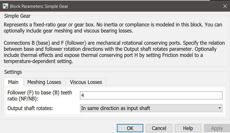
The Simple Gear block is nothing but a fixed-ratio gear or gear box, where follower to base teeth ratio is set as 4.

This simple gear block was then connected to the CVT transmission block along with the CVT gear ratio from another signal builder where the CVT gear ratio was defined. The CVT gear ratio input signal can be seen in the figure below.

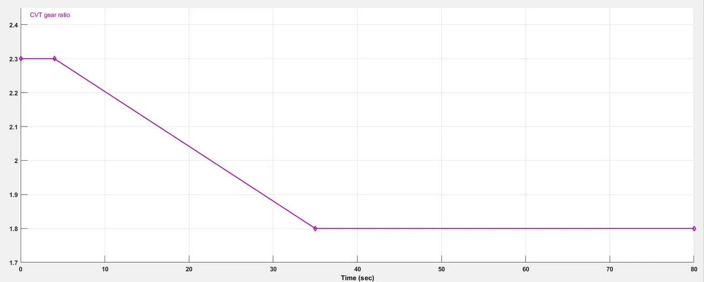
Here it can be seen that the gear ratio is kept at 2.3 for first 4 seconds and then it gradually comes down to 1.8 in the period of next 31 seconds and is constant at 1.8 for next 45 seconds totalling the cycle of 80 seconds. The CVT block built is as shown below.

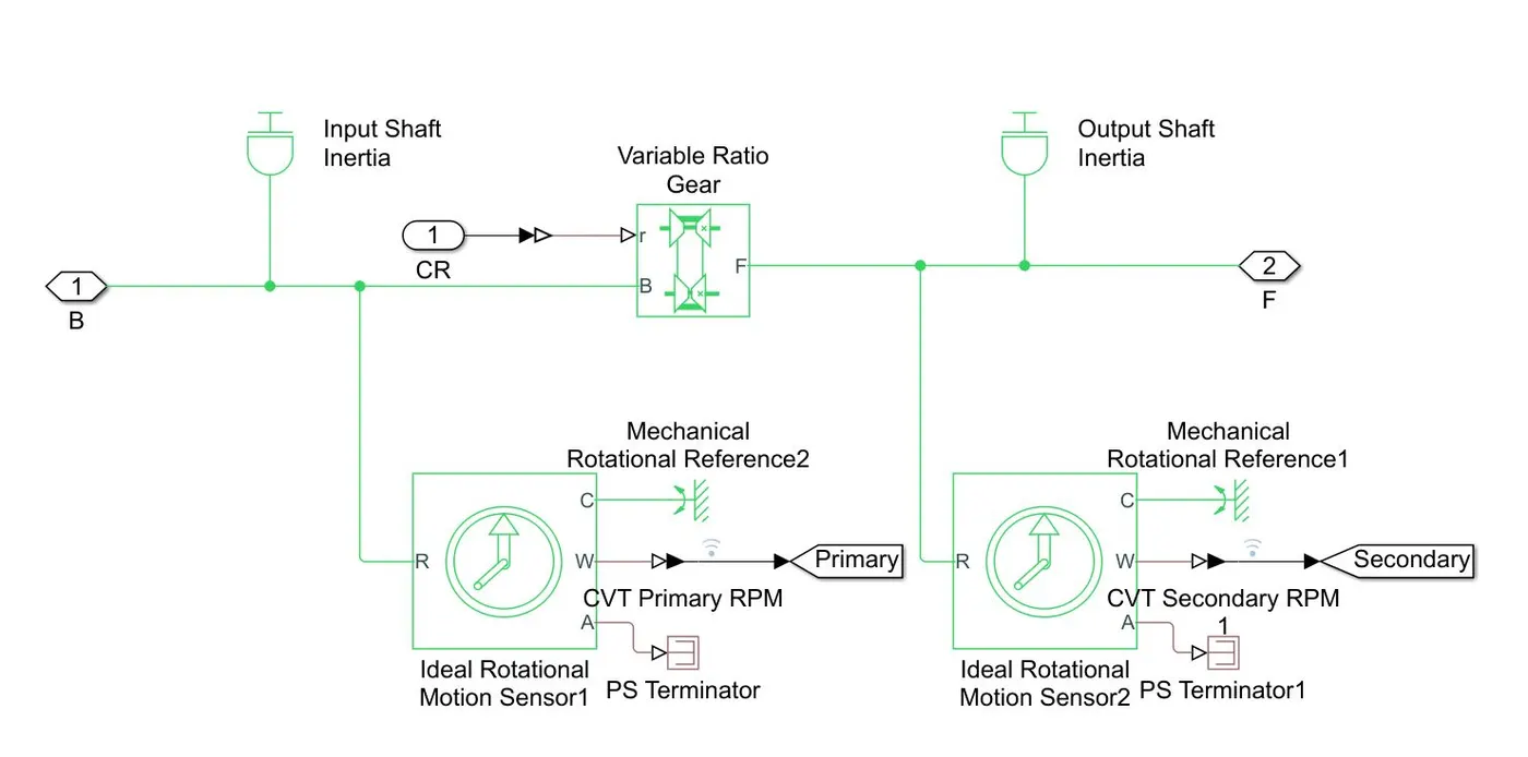
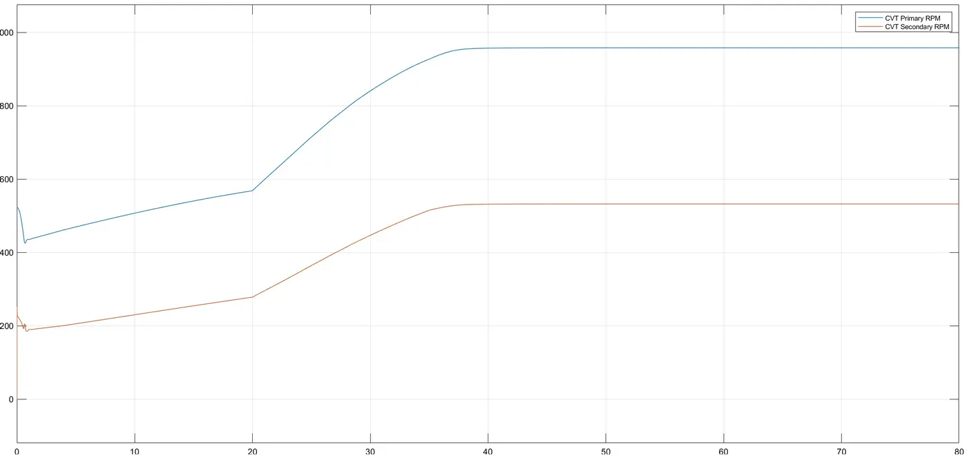
Here the B input port comes from the simple gear block and the CR block is the input from the signal builder for gear ratio. There are two rotational sensors from the primary and the secondary transmission shafts which is basically input and output shaft of the transmission. The variable ratio gear block is added between the two rotational shafts that is the rotational sensors which is nothing but the CVT transmission, this is nothing but the variable ratio transmission implemented by mechanical belt CVT hydraulic or electric transmissions. Here the input port r defines the ratio of input to output angular shaft velocities, which is connected to the gear ratio and the port B is connected to the signal coming from the simple gear which is nothing but the input shaft. The port F is nothing but the output shaft port which then goes to connect to the body of the vehicle in the Simulink block diagram. The primary (input shaft) and the secondary (output shaft) CVT shafts are also given an out output that are later connected to the scope to observe the RPM of these shafts.

Coming to the vehicle body block of the Simscape ATV model. There are two inputs observed to the block which can be seen in the main figure. One input is the brake input and the other input coming from the CVT transmission. The brake input is the input coming from the signal builder where brake signal was provided. The vehicle body block figure is as seen below.

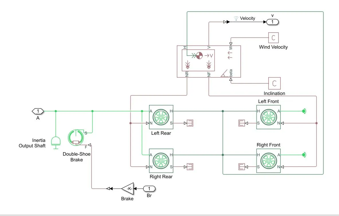
At the input port A is the output shaft of the transmission which gives drive to the wheels can be seen in the figure, which is connected to the output inertia shaft. This then later connects to the rear wheels. The wheels are then connected to the vehicle body.

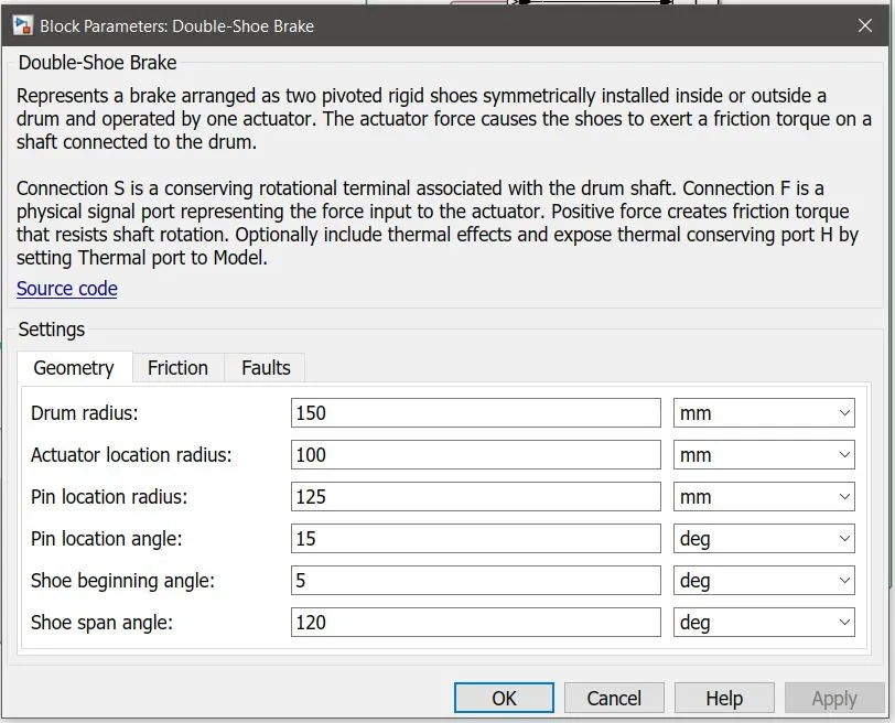
The double shoe brake is the regular drum brake used in most of the vehicles. In the double shoe brake block connection S is a conserving rotational terminal associated with the drum shaft. Connection F is a physical signal port representing the force input to the actuator. Positive force creates friction torque that resists shaft rotation. The Simulink brake input is connected to the Simscape double shoe brake via Simulink PS converter and the parameters of the brake can be seen the figure below.

The vehicle body block as seen below represents a two axle body in longitudinal motion. The block consists of the body weight, aerodynamic drag, weight distribution between axles due to acceleration and road profile and road incline.

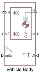
Here connection H is the mechanical translational conserving port associated with the horizontal motion of the vehicle body. The resulting traction motion developed by tires should be connected to this port. Connections V, NF, and NR are physical signal output ports for vehicle velocity (which is observed via scope in the end) and front and rear normal wheel forces, respectively. Wheel forces are considered positive if acting downwards. Connections W and beta are physical signal input ports corresponding to headwind speed and road inclination angle, respectively.

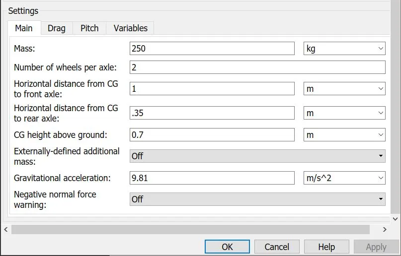
The vehicle body block parameters can be seen below.

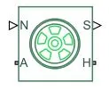
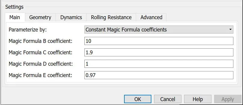
The tires connected to the vehicle are the tires with the magic formula. Here in the tire connection A is the mechanical rotational conserving port for the wheel axle. Connection H is the mechanical translational conserving port for the wheel hub through which the thrust developed by the tire is applied to the vehicle. Connection N is a physical signal input port that applies the normal force acting on the tire. The force is considered positive if it acts downwards. Connection S is a physical signal output port that reports the tire slip. The block parameters for the tire Magic formula can be seen below.

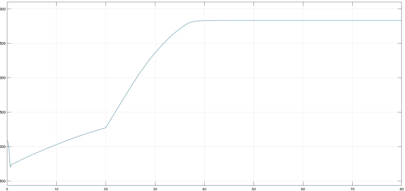
The simulation for this configuration was run for 80 seconds, as the default parameters for this model were given for 80 seconds. The input parameters for break, throttle and CVT gear ratio were seen earlier. The simulation output of this setup can be seen below.

Torque VS Speed (default plot):

Vehicle Speed:

Engine RPM:

Primary and Secondary CVT Shaft Speed:

Part 1.2: ATV Model with Dashboard

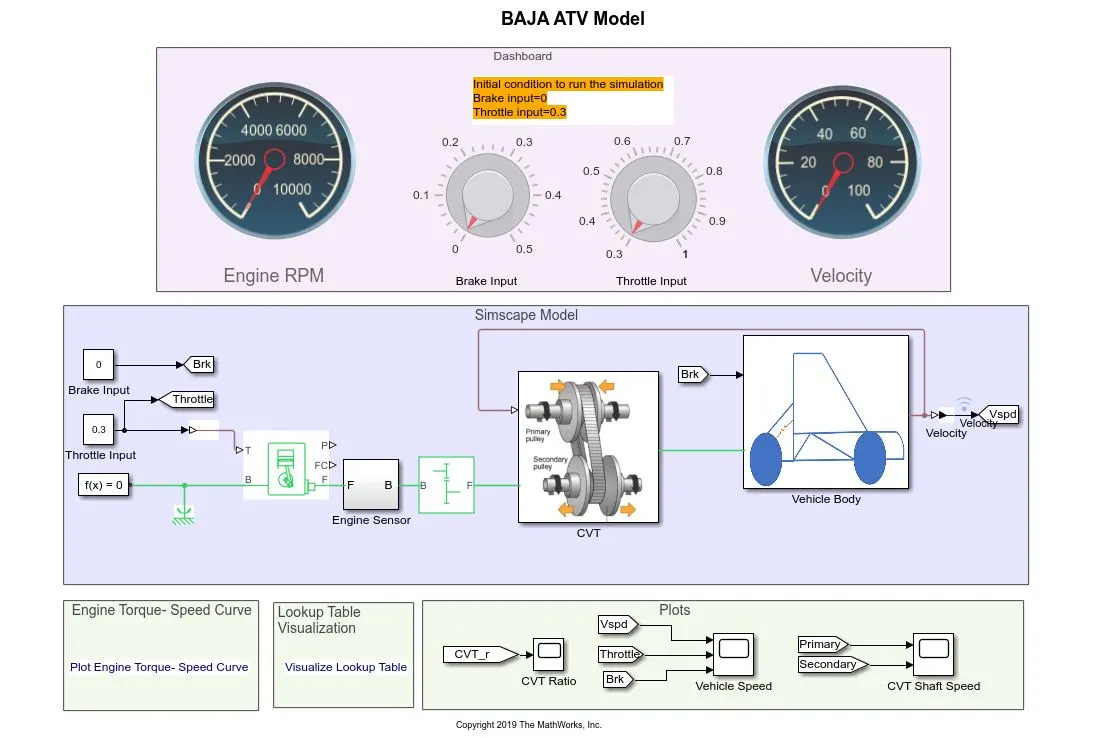
The Simulink model of ATV with dashboard can be seen below.

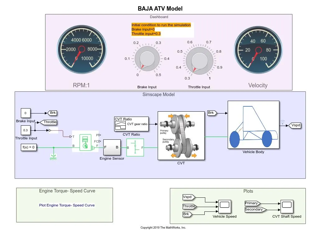
Here as seen in the figure above, the Simscape model was built with the Dashboard similar to vehicle. The remaining vehicle system remains the same as the previous model, the only difference is the manual throttle and brake inputs to be given to observe the outputs. Here the brake and the throttle inputs can be given manually unlike in the previous model where the inputs were given by a signal builder. The Engine RPM gauge and the Velocity gauge displays the changes happening while the vehicle is running. In this model the simulation stop time is defined as “inf” that is infinite time, the simulation only stops when stopped manually. This is to observe what happens to RPM and Velocity of the vehicle when the brake and throttle inputs given to the system via knobs.

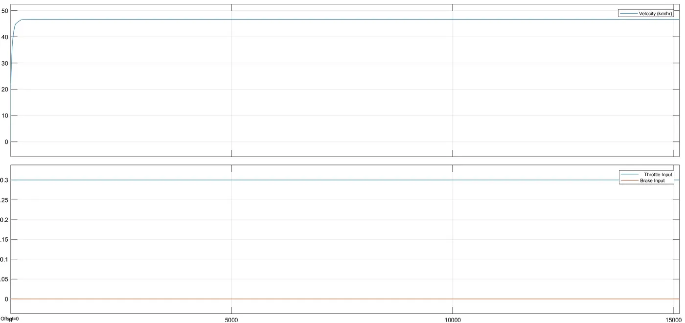
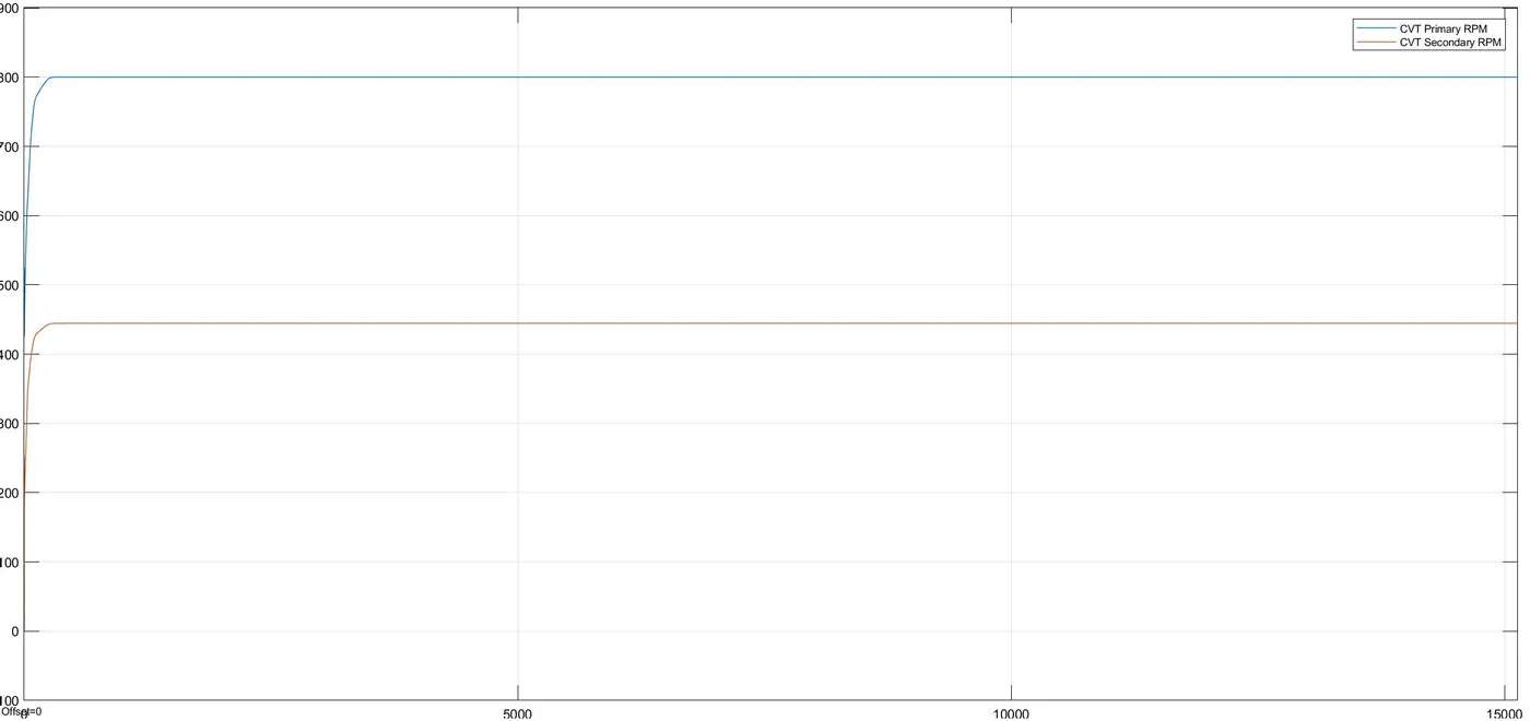
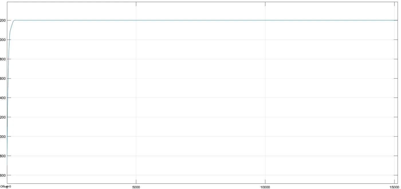
The first simulation was ran keeping the brake and throttle at the default position that is the brake at 0 and throttle at 0.3. The output of the simulation can be seen below.

Vehicle Speed:

CVT Shaft Speed:

Engine RPM:

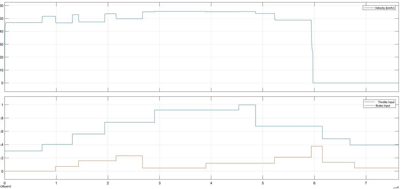
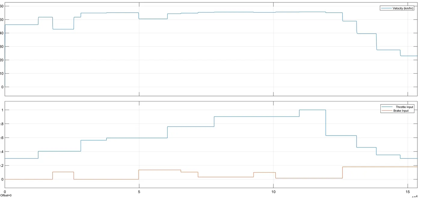
The manual brake and throttle inputs were then given to observe the outputs. The results of the simulation can be seen below.

Vehicle Speed:

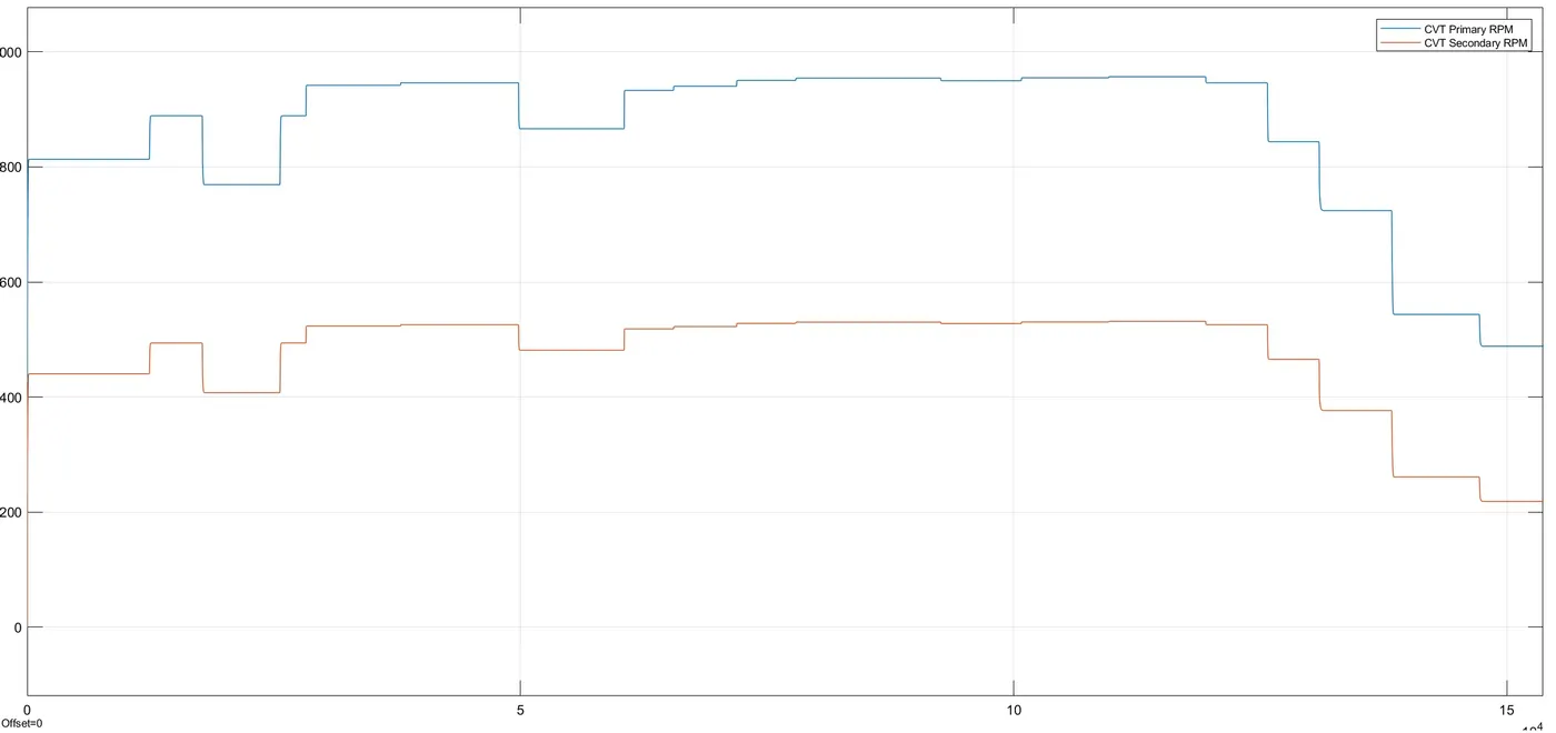
CVT Shaft Speed:

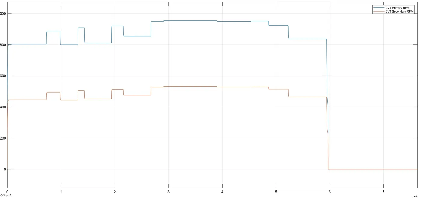
Here the difference in variation of speed of the vehicle and the CVT shaft RPM variation can be seen changing as the brake and throttle inputs differ. The vehicle speed can also be seen changing with the throttle and brake inputs. The CVT shaft RPM can be seen changing. The default CVT primary shaft can be observed at 500 RPM and the secondary shaft at 420 RPM and varies as the throttle and brake inputs varies.

Part 2: BAJA ATV Simulink Models with Lookup table.

Part 2.1: ATV Model without Dashboard.

The ATV model with Lookup table and with out dashboard can be seen below.

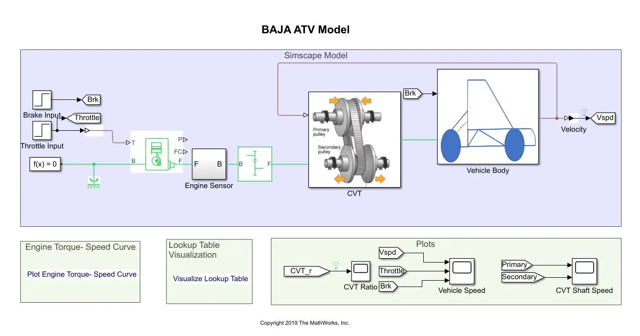
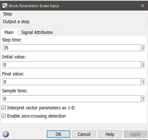
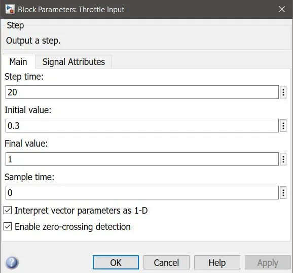
The main difference between the ATV models without Lookup table and with Lookup table is that the CVT transmission ratio, here in the model with the Lookup table there is no input for transmission ratio through Signal builder, a Lookup table is linked in the transmission model whose inputs are in the form of a Lookup table linked in Matlab via external .mat file. Here in this model the throttle and brake inputs are given through step inputs and not via Signal builder. The input block parameters for brake and throttle for this model can be seen below.

Brake input parameters:

Throttle input parameters:

The Lookup table is an array of the data that maps input to output values, thereby approximating a math function. A set of inputs is already present to link it to the model via an external file. If the table is not able to give the explicit required values, then Simulink estimates the output values using the interpolation, extrapolation or rounding off technique [4].

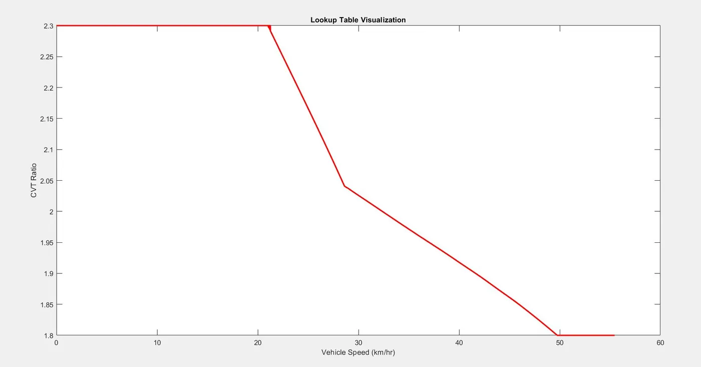
The inputs of the Lookup table can be seen below from the “Visualise Lookup Table” tab under the model, where the graph is Vehicle speed VS CVT Ratio.

The difference in the transmission models with and without lookup tables can be seen below.

The transmission model without Lookup table:

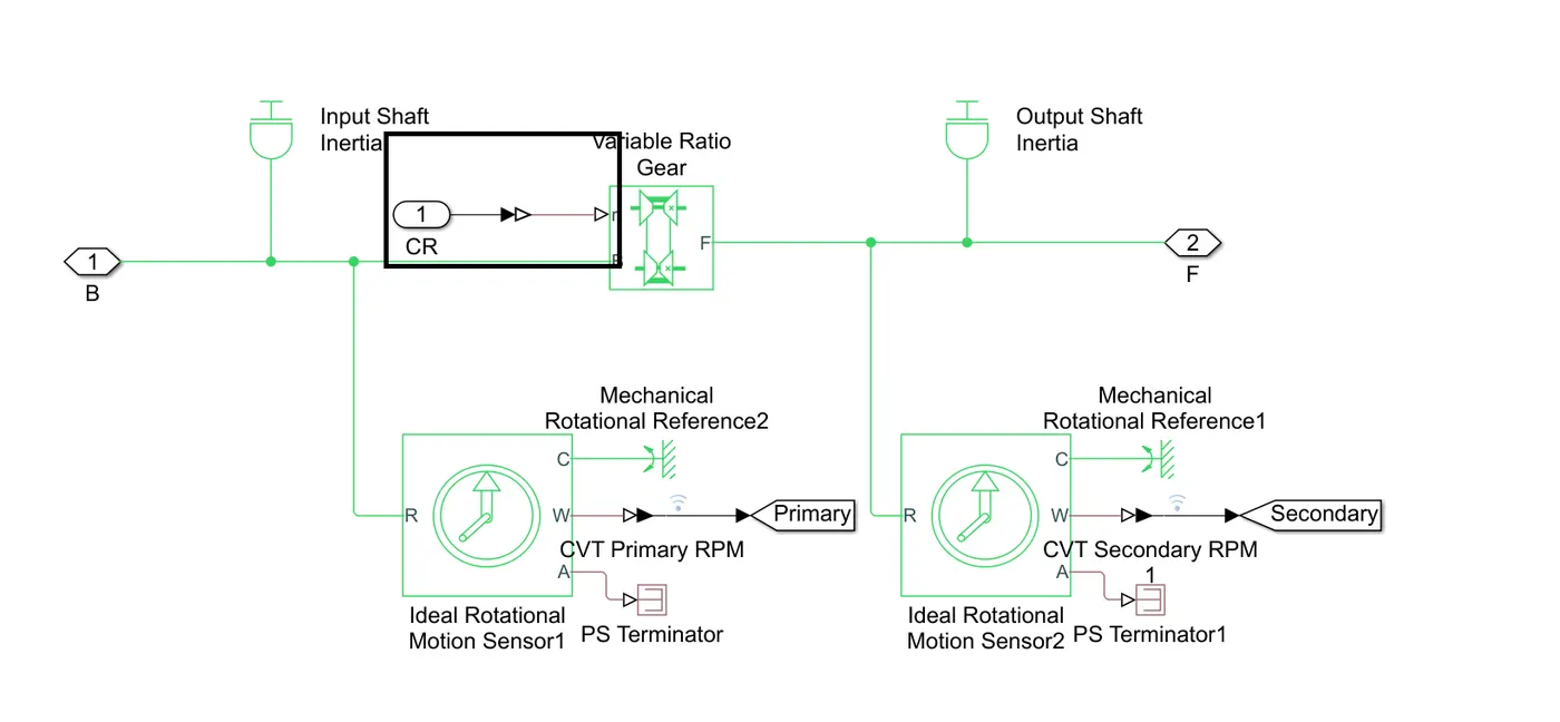
In this model there is direct input of gear ratio from signal builder to the Variable Ratio Gear block.

The transmission model with Lookup table:

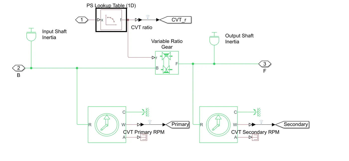
In this model the gear ratio is input via the lookup table data linked directly from .mat external file. The Lookup table file consisted the CVT ratio and vehicle speed, wherein CVT ratio varies based on 1D lookup table.

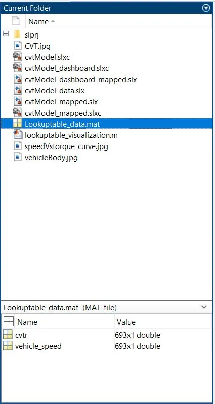
As seen above the Lookup table file can be found with the other files in the folder. The values of “cvtr” and ‘vehicle_speed” are fetched from here. The values in the file can be seen below.

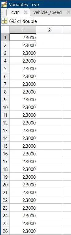
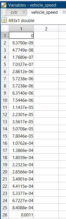
The assigned Lookup table block parameters can be seen below.

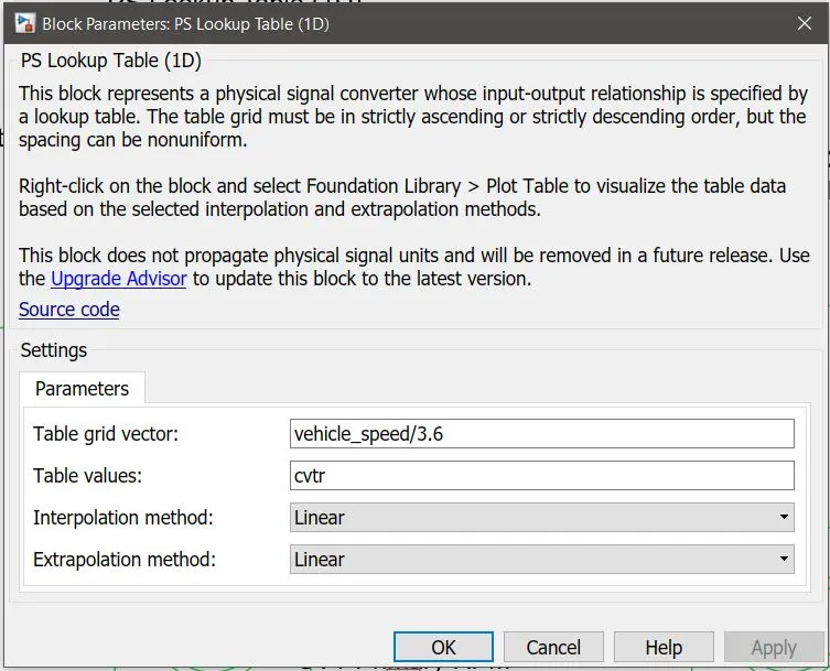
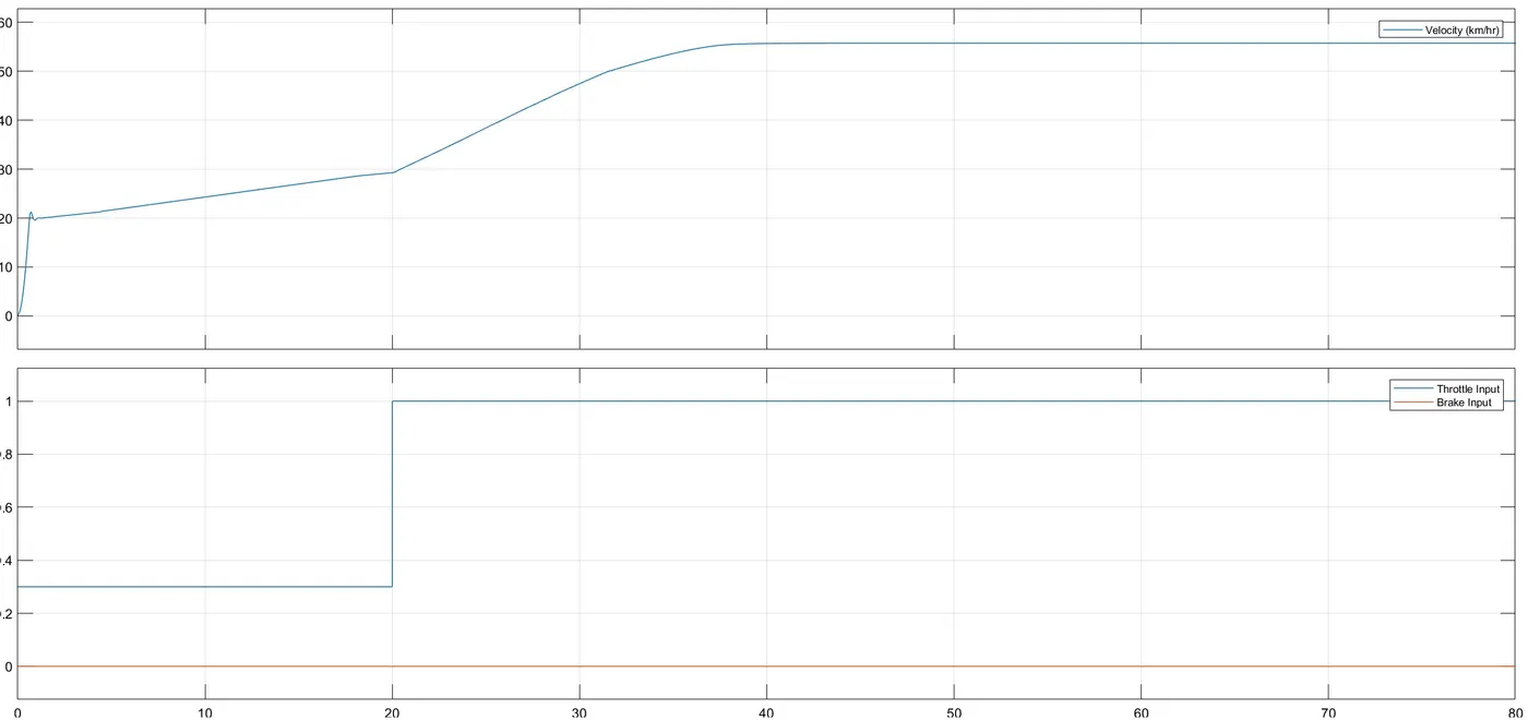
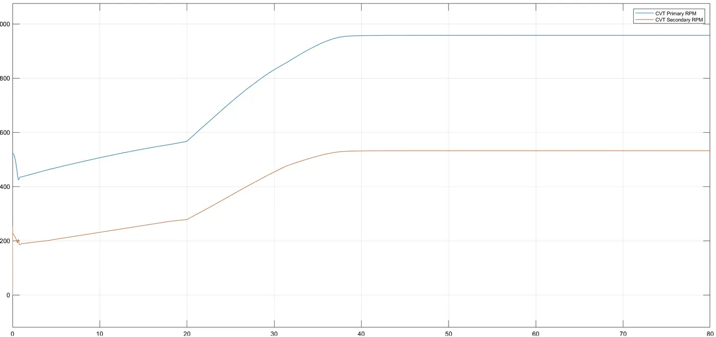
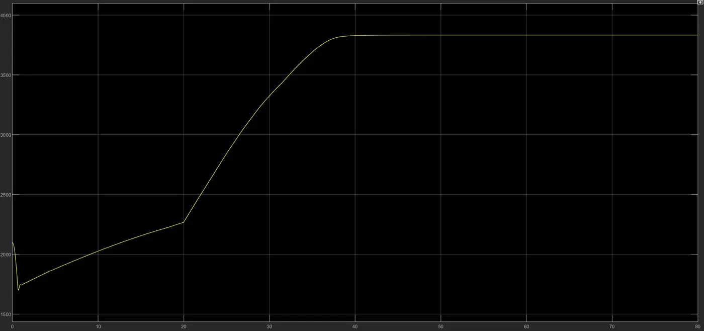
After running the simulation for assigned value of stop time for simulation of 80 seconds, following plots were observed.

Vehicle Speed scope output:

CVT Shaft scope output:

Engine RPM:

CVT Ratio Scope output:

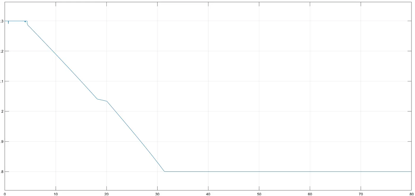
The above output resembles the plot seen previously of CVT Ratio VS Vehicle Speed from Lookup table.

Part 2.2: ATV Model with Dashboard.

The ATV model with dashboard can be seen below.

Vehicle Speed scope output:

CVT Shaft scope output:

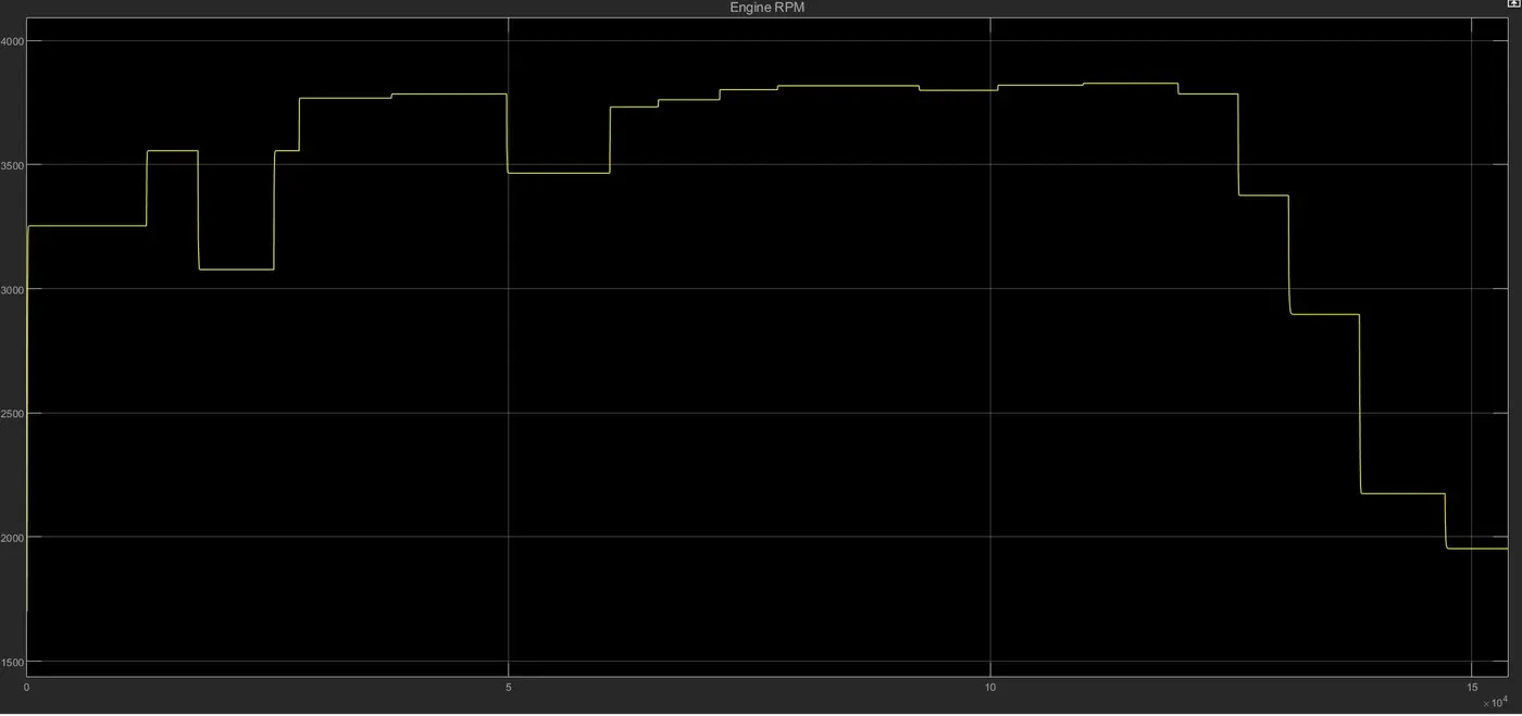
Engine RPM:

CVT Ratio Scope output:

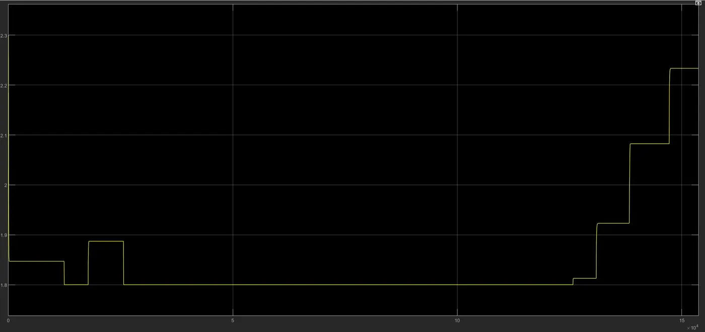
Here in the above graph the difference between the outputs of the CVT Ratio in the models with dashboard and without dashboard can be seen as in the previous model the throttle and brake inputs were predefined and here in the model with dashboard the throttle and brake inputs were applied manually. The transmission ratio can be seen decreasing as the speed rises and the ratio increases as the speed decreases.

Conclusions:

1. It can be concluded that the simulation for BAJA ATV for all four models was successful.
2. CVT Shaft RPM, Engine RPM and Velocity are directly proportional to the throttle input and inversely proportional to the brake input.
3. CVT Primary Shaft speed is greater than the Secondary Shaft speed as they are directly proportional to their shaft diameter respectively.
4. The speed might get zero at a particular resistance of braking.
5. CVT ratio is directly proportional to torque input and inversely proportional to throttle input.

References:

[1] https://en.wikipedia.org/wiki/Baja_SAE

[2] https://www.financialexpress.com/auto/car-news/how-mahindra-baja-sae-india-is-fuelling-passion-among-young-minds-all-that-you-need-to-know-as-a-student/1099983/

[3] https://en.wikipedia.org/wiki/Continuously_variable_transmission

[4] https://in.mathworks.com/help/simulink/ug/about-lookup-table-blocks.html