Project 2
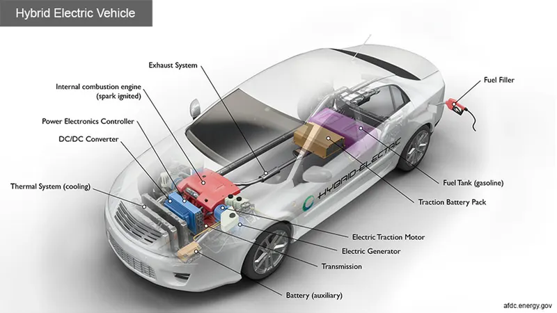
Project 2
development of a forward energy-based fuel consumption model of a P1 hybrid vehicl
Abhishek Anil Patil | 12/04/2022
Objective
Project 2 deals with the development of a forward energy-based fuel consumption model of a P1 hybrid vehicle.
he main goal of this project is to understand the functionality of a P1 hybrid and be able to model it.
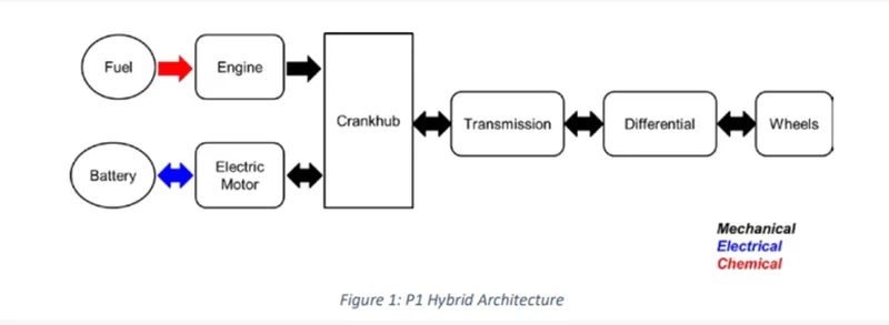
Honda Insight motor and battery are considered for this project. Data is taken from ADVISOR data base developed by NREL, USA. Data provided in the project files.
- Tabulate the fuel economy numbers (kmpl) for UDDS and HWFET cycle. Compare these numbers with the baseline numbers for conventional vehicle model from Project 1.
b. Plot the time trace for engine, transmission input, transmission output and wheel speed on one plot.
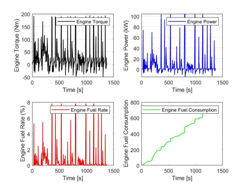
c. Plot engine torque, engine power, fuel rate and fuel consumption using subplots.
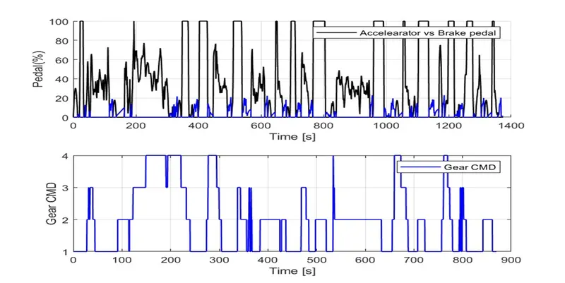
d. Plot accelerator and brake pedal, gear command, vehicle desired and actual speed, vehicle distance using subplots.
e. Plot the engine operating points on the engine fuel map.
f. Plot motor speed, torque, motor input power using subplots.
g. Plot pack voltage, current and SoC using subplots.
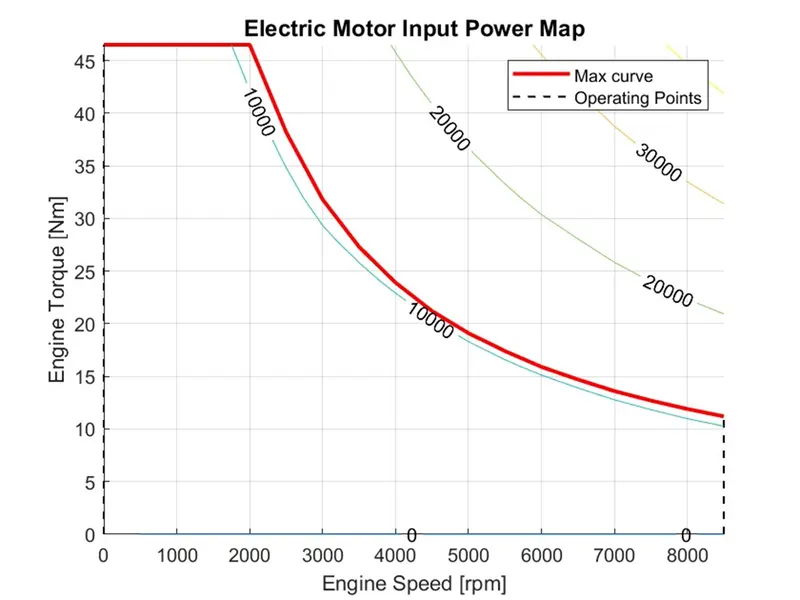
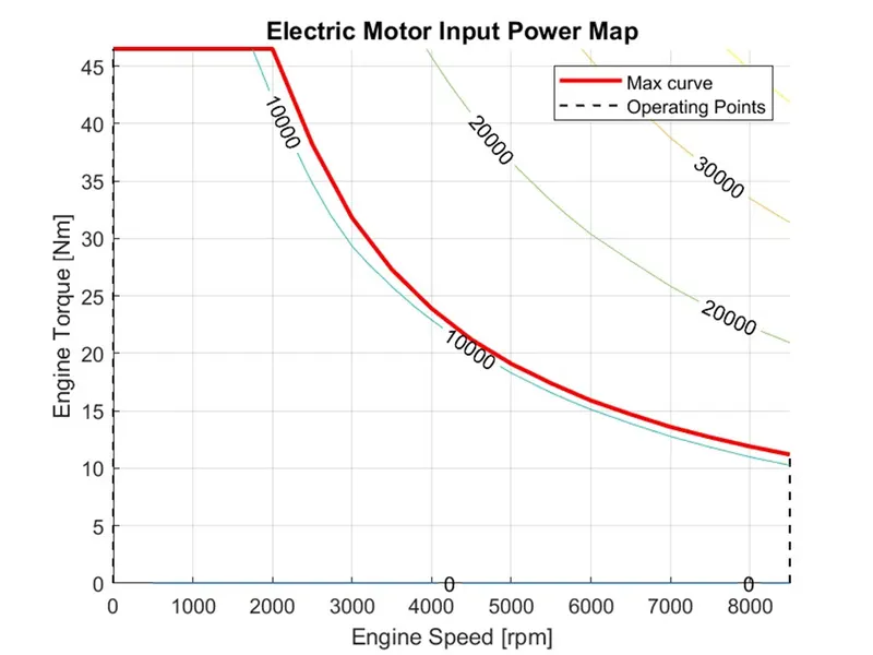
h. Plot the motor operating points on the motor input power map, with the motor max motoring and generating torque curves.
i. Write down appropriate brief comments on each of these plots, describing the vehicle behavior throughout the drive cycle.
j. Generate the plots for both drive cycles
Hybrid Architecture
The brief description of the electric machine connection points is done in the table below.
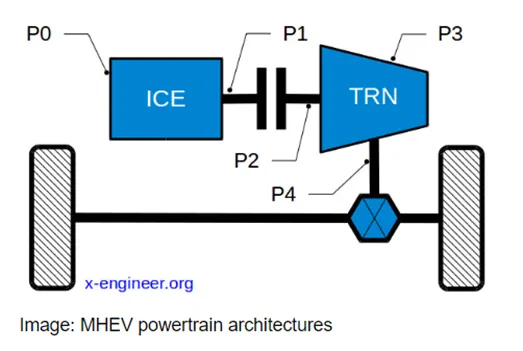
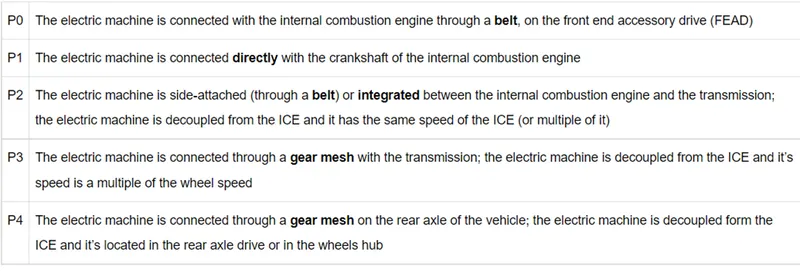
P1 Hybrids
The P1 architecture, with the electric machine connected directly to the crankshaft, is the solution adopted by Honda on their first-generation Integrated Motor Assist (IMA) technology. The electric motor functions as a generator, during vehicle deceleration, as an engine starter, and as a motor (to assist the engine) during vehicle accelerations.
One of the biggest advantages of this solution is that the electric motor can provide higher torque than the BiSG, since there is no belt limitation (due to slip). However, since there is no speed / torque ratio between the electric machine and crankshaft, the torque requirements on the electric motor can be quite demanding.
|
Electric machine performance |
Maximum torque (at crankshaft): up to 34 Nm |
|
Hybrid modes (functions) |
Idle Stop & Start |
|
Advantages |
Higher efficiency |
|
Disadvantages |
Output torque limited by the size of the electric machine |
|
Overall characteristics |
Torque Boosting Capability: High (if electric machine is capable) |
Initialization script
%%%%%%%%%%%%%%%%%%%%%%%%%%%%%%%%%%%%%%%%%%%%%%%%%%%%%%%%%%%%%%%%%%%%%

%% Skill-Lync -> Hybrid Drives Development

% Project 1 - Hybrid Electric Vehicle Model

% By - Ullekh Gambhira


% Description:


%% Initialization File

% Initialization file for loading the variables for the Hybrid Electric vehicle simulation model


%% Vehicle Parameters

M = 1500;       % Vehicle weight [kg]

Cr = 0.015;     % Rolling resistance coefficient

Rw = 0.35;      % Rolling radius [m]

Cd = 0.33;      % Drag coefficient

Af = 2;         % Frontal area [m2]

rhoa = 1.225;   % Air density [kg/m3]

Vwind = 0;      % Wind velocity [kmph]

g = 9.81;       % Gravitational acceleration [m/s2]

theta = 0;      % Slope [deg]

myu_road_tire = 1; % Coefficient of friction between tire - road interface


%% Powertrain Parameters

FDR = 3.73;                         % Final Drive Ratio / Diff Ratio

DiffEff = 0.99;                     % Differential efficiency (assumed independent of operating conditions)


NumGear = 4;                        % Number of gears in transmission

TransGear = [1:NumGear];            % Transmission Gears

TransRatio = [3.06, 1.62, 1, 0.7];  % Corresponding Transmission ratios

TransEff = 0.90;                    % Transmission efficiency (assumed independent of operating conditions)


TC_SR = [0, .5, .6, .7, .8, .87, .92, .94, .96, .97, 1];   % Torque Converter Speed Ratio (Matlab default) -> TurbSpd/PumpSpd

TC_TR = [2.232, 1.5462, 1.4058, 1.2746, 1.1528, 1.0732, 1.0192, 1, 1, 1, 1];   % Torque Converter Torque Ratio (Matlab default) -> TurbTrq/PumpTrq

TC_Cf = 1e-4 * [.72558, .66322, .63463, .59042, .51331, .4144, .29287, .22444, .12186, .04386, 0]; % Torque Converter Capacity Factor (Matlab default) -> PumpTrq/PumpSpd^2 [Nm/rpm^2]


load Vehicle_Data/Engine_data_1_9L_Saturn_95kW

load Vehicle_Data/Trans_Shift_map

load Vehicle_Data/EM_Honda_Insight_10kW

load Vehicle_Data/ESS_NiMH6


ESS_init_soc = 0.8;

ESS_soc_max = 0.9;

ESS_soc_min = 0.6;


%% Driver Parameters

Kp = 10;                    % P gain for driver PI model

Ki = 1;                     % I gain for driver PI model

Drive_Cycle_Select = 2;     % Drive cycle selection


% Drive cycle values in m/s


if Drive_Cycle_Select == 1

    load DriveCycles/UDDS;


elseif Drive_Cycle_Select == 2

    load DriveCycles/HWFET;


elseif Drive_Cycle_Select == 3

    load DriveCycles/FTP;


elseif Drive_Cycle_Select == 4

    load DriveCycles/US06;


elseif Drive_Cycle_Select == 5

    load DriveCycles/NEDC;


elseif Drive_Cycle_Select == 6

    load DriveCycles/WLTP;


end


time_end = cyc_time(end);

vel_end = cyc_vel(end);
Simulink model
Layout
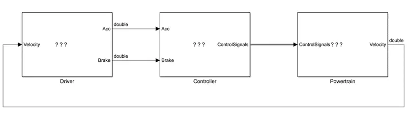
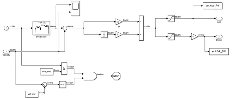
Driver
It contains a PI controller to get the accelerator and brake pedal signals depending upon the drive cycle requirements.
Controller
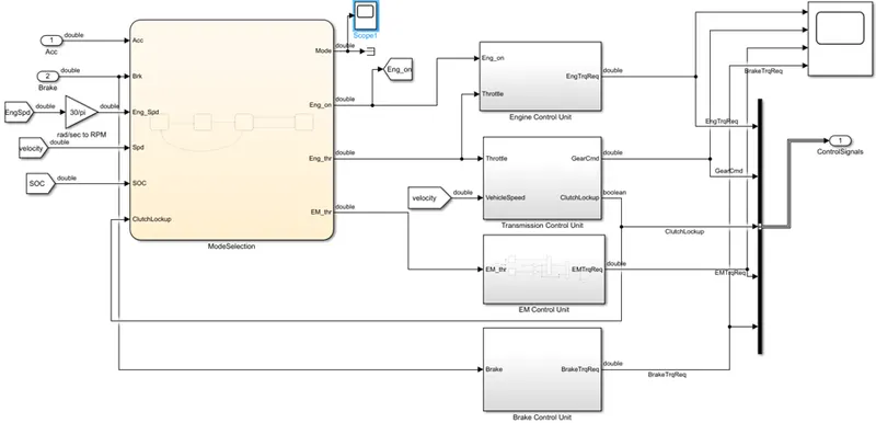
This is the brains of the vehicle
It generates desired engine and motor torque signals, gear signals, which are fed to the powertrain.
State flow – Mode Selection
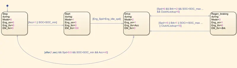
The chart has 4 states, namely Stop, Start, Drive and Regen Braking.
These states are indicated by a mode going from 0 to 3.
Eng_on represents whether the engine is on or off
Eng_thr and EM_thr are for the engine and EM throttle respectively
States
The first state indicates that the vehicle has stopped.
The second state indicates starting phase which is why only EM is used.
The third state is the driving state where the engine is on and the EM is off
The fourth state indicates regenerative braking where the engine throttle is o and the EM throttle is equivalent to the brake pedal signal.
Transitions
State 1 – 2
Acc>1 || SOC<SOC_min
For the starting phase if the accelerator signal is more than 1 or if the SOC has fallen below the minimum value
State 2 – 3
Eng_Spd>Eng_idle_spd
Between the starting and driving phase the transitions happens when the engine speed is greater than the engine speed at idle state.
State 3 - 4
Spd>6 && Brk>=2 && SOC<SOC_max ... && ClutchLockup>0
From driving to regenerative braking, if speed and brake signal are above certain values and SOC is less than its max value and the Clutch lock up is more than 0.
State 4 – 3
Spd<=5 || Brk<1 || SOC>=SOC_max ... || ClutchLockup==0
If any of the previous conditions are not met then the vehicle will go from regen braking to the driving state.
State 3-1
after(1,sec) && Spd<0.5 && SOC<SOC_min && Acc==0
Driving and stop condition, transition is indicated by checking the Speed values are below a certain threshold and the SOC value is less than its minimum and the acceleration is 0. This is checked after every second.
Engine Control Unit
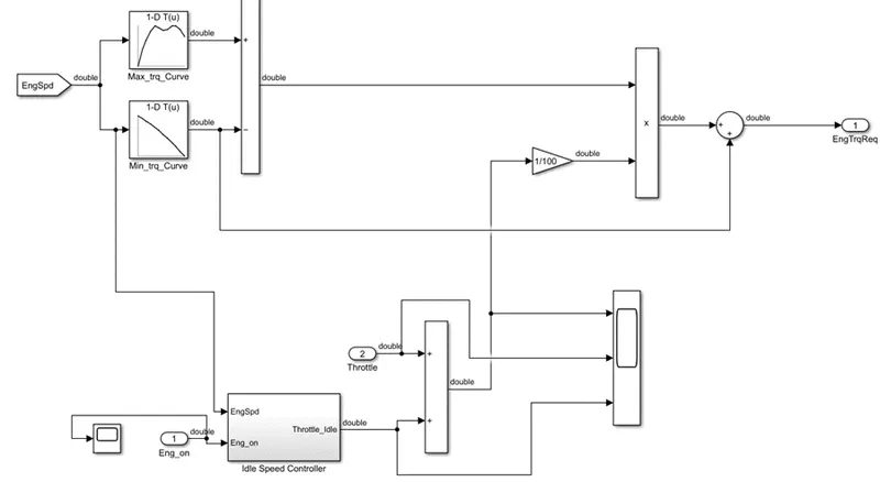
The idle speed controller keeps the speed above the idle speed and make sure that the engine is idling provided that the engine is on.
The accelerator pedal from the driver unit provides the throttle signal as an input.
It has two look up tables for maximum and minimum torque curves for various speed values.
The input to the tables is the engine speed. This input along with the throttle and idle speed controller signals are multiplied together to get the required engine torque.
Transmission Control Unit
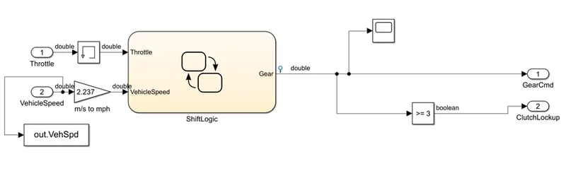
It uses state flow to determine gear shifting.
Velocity and throttle are taken as inputs and the gear used currently is given as an output
Shift Logic
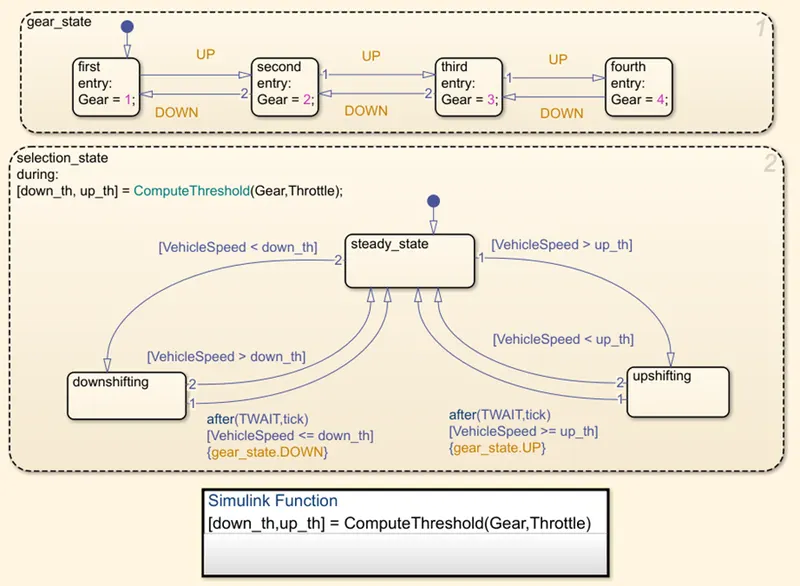
The Gear_state state block decides which gear to shift to using the UP and DOWN decision arrows.
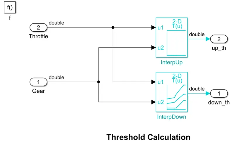
The decision is done by the selection_state state block. Using the ComputeThreshold Simulink function it calculates the values of up_th and down_th which decide whether the gear state should be up or down.
Threshold Function
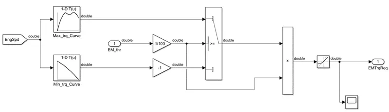
Electric Motor control Unit
Brake Control Unit
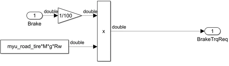
The brake torque is calculated analytically and multiplying it with the brake signal, the magnitude of the brake torque which is required is generated.
The above three signals are connected to a bus, which is transferred to the powertrain block
Powertrain Model
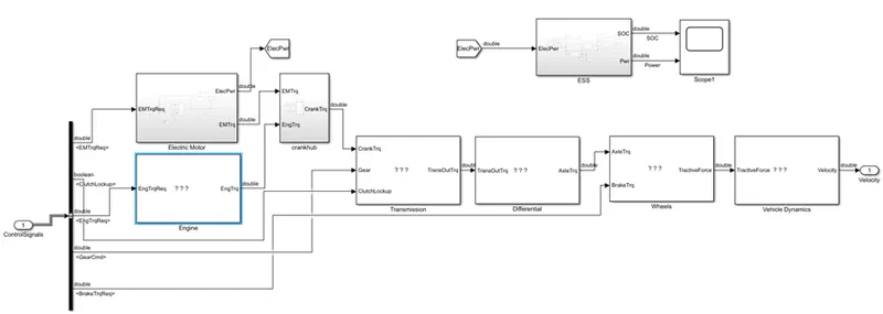
Every component of the system that converts power into movement is included in the power train block.
Engine
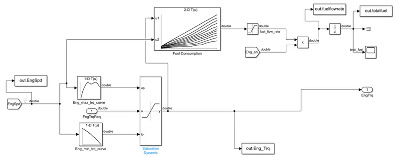
The max and min torque curves act as upper and lower bounds for the engine torque signal which is given to the 2D look up table of fuel consumption. The look up table gives the fuel flow rate and the integrator gives the total fuel consumed until that point.
Electric Motor
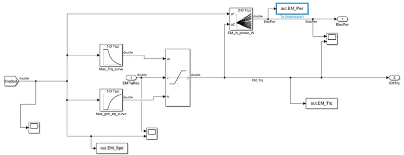
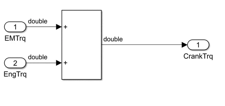
Crank hub
Transmission
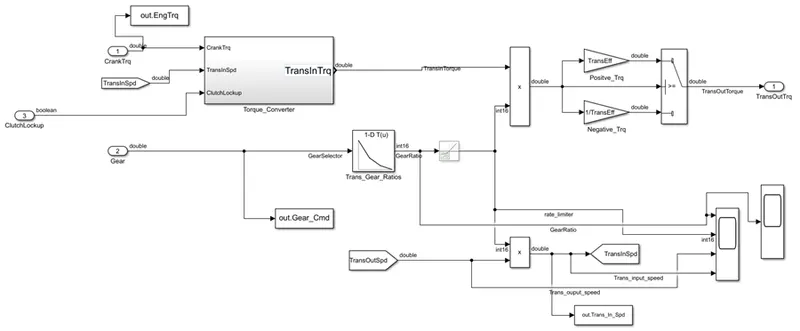
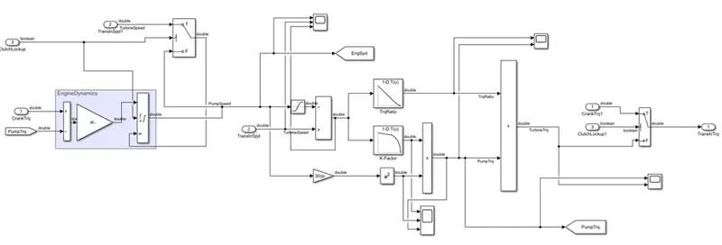
The engine torque, transmission speed and the clutch lock up signal go into the torque converter.
The gear output signals are sent to the transmission gear ratio look up table.
The gear ratio is then multiplied with the transmission torque and transmission efficiency to get the transmission output torque.
The gear ratio is also multiplied with the transmission speed to get the transmission output speed.
Torque Converter
Differential
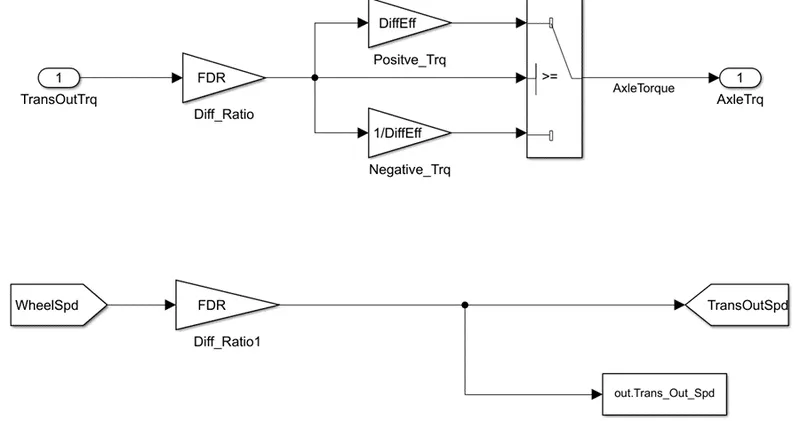
The wheel speed is multiplied by the differential ratio to get the output speed
Transmission torque is further multiplied or divided by the differential efficiency depending on whether the torque is positive or negative respectively.
The output is the axle torque.
Wheels
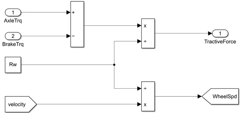
The brake torque is subtracted from the axle torque to get the net torque, which is then divided by the wheel radius to get the tractive force.
The velocity is divided by the wheel radius to get wheel speed.
Vehicle Dynamics
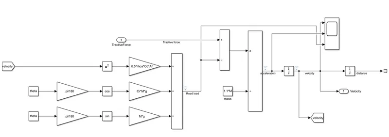
The dynamic equation for calculating the road load is

This equation is represented using the various mathematical blocks, which after integrating gives us the velocity
Estimates Storage System model
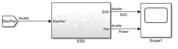
The input to the subsystem is the Electric Power.
The outputs are the SOC and the power.
Subsystem ESS
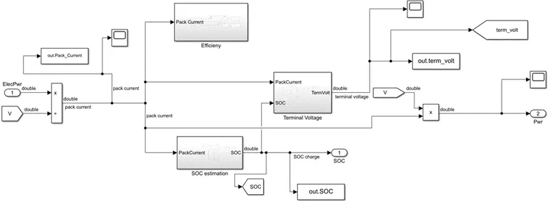
The pack current is calculated by dividing the power by the voltage.
The SOC estimation subsystem is used to calculate the SOC which is used as input to the terminal voltage subsystem.
The battery voltage multiplied by the pack current gives the power.
SOC estimation
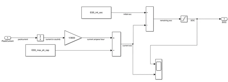
The pack current is integrated to get current in coulomb which is then divided by 3600 to get current in Ampere-hour.
This is divided by the max ampere hour capacity to get the current soc.
This after subtracting from the initial battery soc will give us the SOC value.
terminal voltage
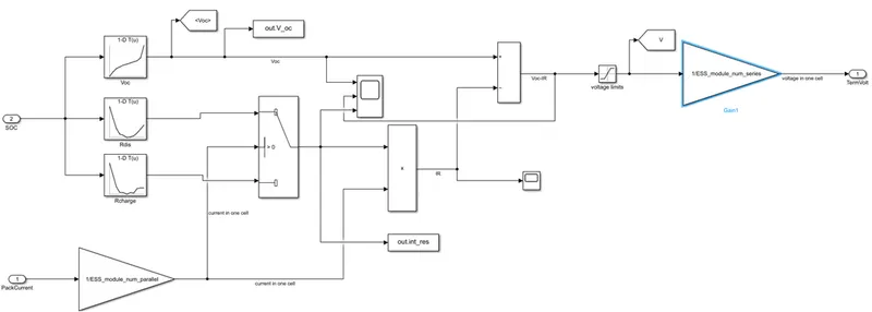
The pack current is divided by the no of parallel modules in the battery packs as the current in parallel is divided while the voltage remains the same. This gives us the current in one cell.
This current is connected to the control port of the switch block. The other two blocks are connected to the charging and discharging resistance look up tables. The criteria being, if the current is greater than zero than cell is discharging otherwise the cell is charging.
The input to the lookup tables is the SOC. The third lookup table gives us the open circuit voltage.
The switch block decides the internal resistance of the cell (R). This is multiplied by the current to get (IR). This when subtracted from the open circuit voltage gives us the battery pack voltage.
This battery pack voltage is divided but the no of modules in series to get the terminal voltage.
Post-Processing Script
%%%%%%%%%%%%%%%%%%%%%%%%%%%%%%%%%%%%%%%%%%%%%%%%%%%%%%%%%%%%%%%%%%%%%

%% Skill-Lync -> Hybrid Drives Development

% Project 1 - Hybrid Electric Vehicle Model

% By - Ullekh Gambhira


% Description:

% The following file is to used with the Initialization file and Simulink

% results for post-processing of the data.

% The file is incomplete, has some examples of how the data is imported

% into a readable format, data analysis and plotting examples.

% Based on the project task, use commands in a similar format as given

% below, to analyse the data and generate required plots.

% You can change variable names if desired


%% Post-Processing File

%  File for post-processing the Conventional vehicle simulation model data


%% Renaming variables


clc;

close all;


Time = out.tout;

Acc_Pdl = out.Acc_Pdl;                              % Accelerator pedal [%]

Brk_Pdl = out.Brk_Pdl;                              % Brake pedal [%]

Gear_Cmd = out.Gear_Cmd;                            % Transmission gear

Trans_In_Spd = out.Trans_In_Spd*30/pi;              % Transmission input speed [rpm]

Trans_Out_Spd = out.Trans_Out_Spd*30/pi;            % Transmission output speed [rpm]

Eng_Trq = out.EngTrq.Data(:,1);                     % Engine brake torque [Nm]

Eng_Fuel_Consump = out.totalfuel.Data(:,1);         % Engine fuel consumption [g]

Veh_Dist = out.VehDist.Data(:,1)/1000;              % Distance traveled by vehicle [km]

Veh_Spd = out.VehSpd.Data(:,1)*(18/5);              % Vehicle speed [kmph]

Eng_Fuel_rate = out.fuelflowrate.Data(:,1);         % Engine Fuel Rate %

Wheel_Spd = out.WheelSpd.Data(:,1)*30/pi;           % Wheel Speed

EM_Pwr = out.EM_Pwr.Data(:,1);                      % Electric motor power

EM_Trq = out.EM_Trq.Data(:,1);                      % Electric motor torque

EM_Spd = (18/5)*out.EM_Spd.Data(:,1);               % Electric motor speed [kmph]

Term_volt = out.term_volt.Data(:,1);                % Terminal voltage

SOC = out.SOC.Data(:,1);                            % state of charge

Pack_Current = out.Pack_Current.Data(:,1);          % Pack Current

Eng_Spd = out.EngSpd.Data(:,1)*(30/pi);             % Engine Speed RPM


%% Data Analysis


Eng_Pwr = Eng_Spd.*Eng_Trq.*((pi/30)/1000);                      % Engine brake power [kW]

rho_petrol = 0.7197;                                             % Density of petrol [kg/L]

kmpl = Veh_Dist(end)/(Eng_Fuel_Consump(end)/1000/rho_petrol);    % Fuel economy [kmpl]

fprintf('fuel comsumption [Kmpl] = %f',kmpl);


%% Plotting vehicle characteristics time trace


figure('Name','transmission IN/OUT speed')

hold on

plot(Time, Trans_In_Spd, 'linewidth', 1, 'Color', 'black');

plot(Time, Trans_Out_Spd, 'linewidth', 1, 'Color', 'red');

plot(Time, Wheel_Spd, 'linewidth', 1, 'Color', 'green');

plot(Time, Eng_Spd, 'linewidth', 1, 'Color', 'blue');

ylabel('Speed [rpm]')

xlim([0, Time(end)]);

ylim([0, 6000]);

legend('Trans Input','Trans Output','Wheel Speed','Engine Speed');


%% Plotting Engine charactesticks

figure('Name','Engine charactesticks');

subplot(2,2,1);

plot(Time, Eng_Trq, 'linewidth', 1, 'Color', 'black');

xlabel('Time [s]');

ylabel('Engine Torque (Nm)');

legend('Engine Torque');

grid on;


subplot(2,2,2);

plot(Time, Eng_Pwr, 'linewidth', 1, 'Color', 'blue');

xlabel('Time [s]');

ylabel('Engine Power (kW)');

legend('Engine Power');

grid on;


subplot(2,2,3);

plot(Time, Eng_Fuel_rate, 'linewidth', 1, 'Color', 'red');

xlabel('Time [s]');

ylabel('Engine Fuel Rate (%)');

legend('Engine Fuel Rate');


subplot(2,2,4);

plot(Time, Eng_Fuel_Consump, 'linewidth', 1, 'Color', 'green');

xlabel('Time [s]');

ylabel('Engine Fuel Consumption');

legend('Engine Fuel Consumption');


%% Plotting Fuel Economy

figure('Name','Fuel Economy ');

plot(Time, Eng_Fuel_Consump, 'linewidth', 1, 'Color', 'r');

xlabel('Time [s]');

ylabel('Engine Fuel Consumption [kmpl]');

grid on;


%% Plotting Accelerator brake pedals and gear CMD


figure('Name','Accelerator,brake,gear');

subplot(2,1,1);

hold on;

plot(Time, Acc_Pdl, 'linewidth', 1, 'Color', 'black');

plot(Time, Brk_Pdl, 'linewidth', 1, 'Color', 'blue');

xlabel('Time [s]');

ylabel('Pedal(%)');

legend('Accelearator vs Brake pedal');

grid on;


subplot(2,1,2);

plot(Time(1:height(Gear_Cmd)),Gear_Cmd, 'linewidth', 1, 'Color', 'blue');

xlabel('Time [s]');

ylabel('Gear CMD');

legend('Gear CMD');

grid on;


%% Plotting Gear CMD wrt speed and distance


figure('Name','Gear command wrt Vehicle speed and distance');


subplot(2,1,1);

plot(Veh_Spd(1:height(Gear_Cmd)), Gear_Cmd, 'linewidth', 1, 'Color', 'blue');

xlabel('vehicle speed (kmph)');

ylabel('Gear CMD');

title('Vehicle Speed vs gear CMD');

grid on;


subplot(2,1,2);

plot(Veh_Dist(1:height(Gear_Cmd)), Gear_Cmd, 'linewidth', 1, 'Color', 'green');

xlabel('Vehicle Distance');

ylabel('Gear CMD');

title('Vehicle Distance vs gear CMD');

grid on;


%% Plotting engine operating points on engine fuel map


figure('Name','Engine Operating Points');


hold on

grid on

title('Engine Operating Points','fontsize',12);

p1=plot(Eng_map_spd*30/pi,Eng_max_trq,'linewidth',2,'color','r');

p2=line([Eng_map_spd(end)*30/pi Eng_map_spd(end)*30/pi],[0 Eng_max_trq(end)]);

set(p2,'linewidth',1,'linestyle','--','color','k');

p3=line([Eng_map_spd(1)*30/pi Eng_map_spd(1)*30/pi],[0 Eng_max_trq(1)]);

set(p3,'linewidth',1,'linestyle','--','color','k');

[c,h] = contour(Eng_map_spd'*30/pi,Eng_map_trq,Eng_fuel_map');

clabel(c,h);

xlabel('Engine Speed [rpm]');

ylabel('Engine Torque [Nm]');

title('Engine Fuel Consumption Map [g/s]');

legend([p1 p3],{'Max curve','Operating Points'});

axis([Eng_map_spd(1)*30/pi Eng_map_spd(end)*30/pi 0 Eng_map_trq(end)]);


%% Plotting SOC, pack Current and terminal voltage


figure('Name','SOC, Pack Current and Terminal Voltage');


subplot(3,1,1);

plot(Time, Pack_Current, 'linewidth', 1, 'Color', 'blue');

xlabel('Time[s]');

ylabel('Pack Current [A]');

title('Pack Current');

grid on;


subplot(3,1,2);

plot(Time, SOC, 'linewidth', 1, 'Color', 'red');

xlabel('Time[s]');

ylabel('State of Charge [%]');

title('State of Charge');

grid on;


subplot(3,1,3);

plot(Time, Term_volt, 'linewidth', 1, 'Color', 'm');

xlabel('Time[s]');

ylabel('Terminal Voltage [V]');

title('Terminal Voltage');

grid on;


%% Plotting Motor speed, motor torque , motor input power


figure('Name','Motor speed, motor torque , motor input power');


subplot(3,1,1);

plot(Time, EM_Pwr, 'linewidth', 1, 'Color', 'blue');

xlabel('Time [s]');

ylabel('Electric Motor Power [W]');

title('Electric Motor Power');

grid on;


subplot(3,1,2);

plot(Time, EM_Trq, 'linewidth', 1, 'Color', 'red');

xlabel('Time [s]');

ylabel('Electric Motor Torque [Nm]');

title('Electric Motor Torque');

grid on;


subplot(3,1,3);

plot(Time, EM_Spd, 'linewidth', 1, 'Color', 'm');

xlabel('Time [s]');

ylabel('Electric Motor Speed [RPM]');

title('Electric Motor Speed');

grid on;


%% Plotting engine operating points on engine fuel map


figure('Name','Electric Motor Operating Points');


hold on

grid on

title('Electric Motor Operating Points','fontsize',12);

p1=plot(EM_map_spd*30/pi,EM_max_trq,'linewidth',2,'color','r');

p2=line([EM_map_spd(end)*30/pi EM_map_spd(end)*30/pi],[0 EM_max_trq(end)]);

set(p2,'linewidth',1,'linestyle','--','color','k');

p3=line([EM_map_spd(1)*30/pi EM_map_spd(1)*30/pi],[0 EM_max_trq(1)]);

set(p3,'linewidth',1,'linestyle','--','color','k');

[c,h] = contour(EM_map_spd'*30/pi,EM_map_trq,EM_inpwr_map');

clabel(c,h);

xlabel('Engine Speed [rpm]');

ylabel('Engine Torque [Nm]');

title('Electric Motor Input Power Map');

legend([p1 p3],{'Max curve','Operating Points'});

axis([EM_map_spd(1)*30/pi EM_map_spd(end)*30/pi 0 EM_map_trq(end)]);
Results
Fuel Economy
UDDS
Project 1

Project2

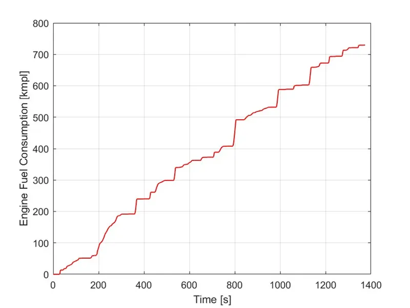
The fuel economy numbers are greater for the conventional vehicle model than the P1 hybrid EV because of the implementation of the Electric motor and the P1 hybrid architecture.
HWFET
Project 1
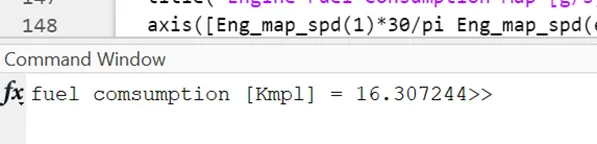
Project 2

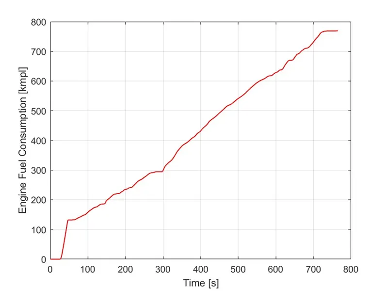
The fuel economy numbers are higher for highway driving as compared to urban city driving because of the lack of traffic which prevent any start stops.
Speeds
UDDS
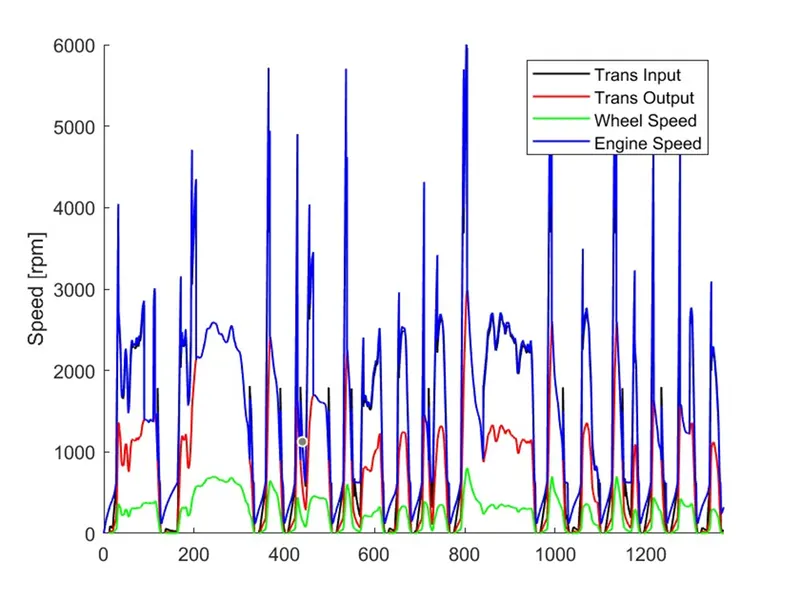
HWFET
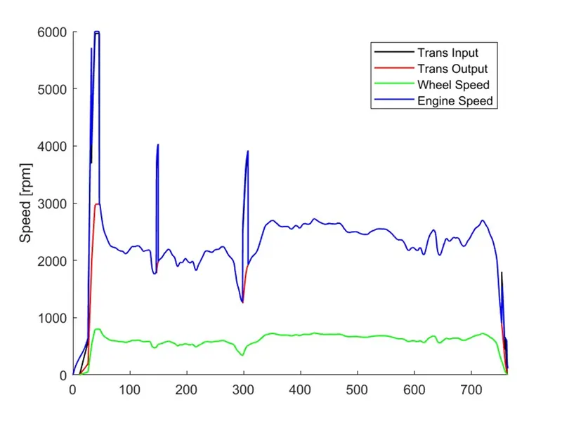
Speeds fluctuate more in urban drive cycle because of traffic intensity which causes the vehicle to start and stop at multiple places.
Engine characteristics
UDDS
HWFET
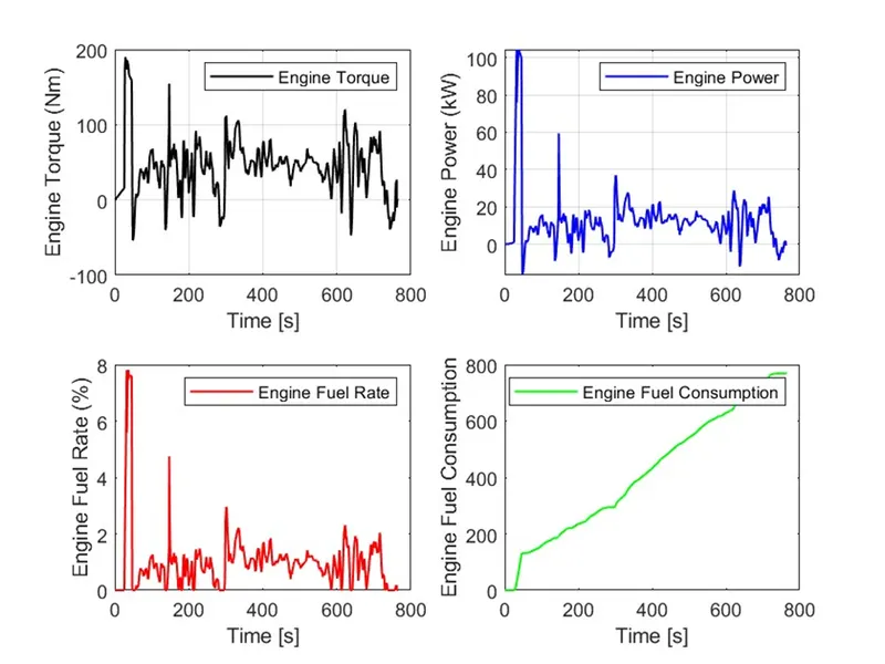
Power and torque for UDDS is more because of the drive cycle start stop nature as compared to HWFET.
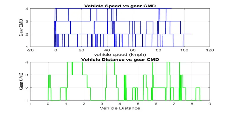
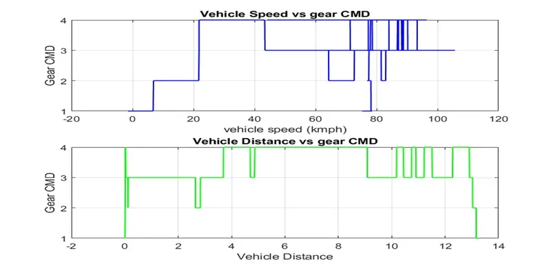
Gear characteristics
UDDS
HWFET
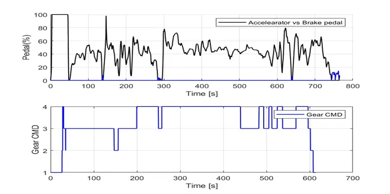
The accelerator and brake pedals fluctuate a lot in UDDS cycle because of frequent start-stops.
HWFET operates mostly in 3- 4 gear whereas the UDDS varies all over the place.
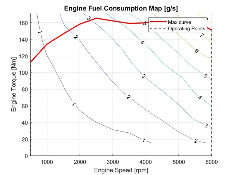
Engine Operating Points
UDDS
HWFET
Motor Characteristics
UDDS
HWFET
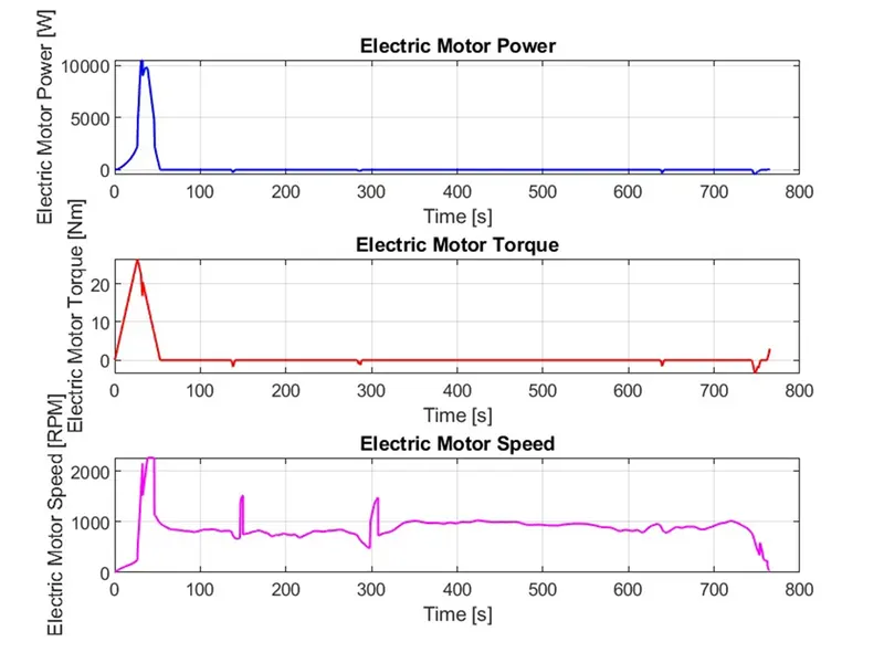
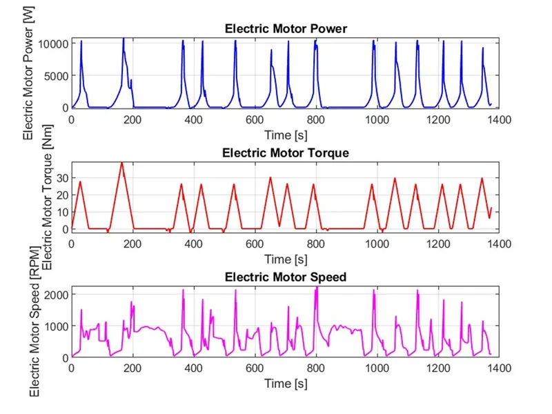
The motor in P1 hybrid is used as engine crank which is why It is used more in urban cycle because of all the start-stops.
The motor is used only at the start of the highway cycle as it never brakes until the end of the cycle.
SOC, current and voltage
UDDS
HWFET
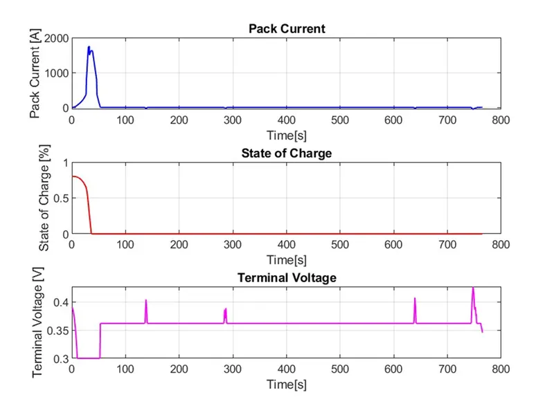
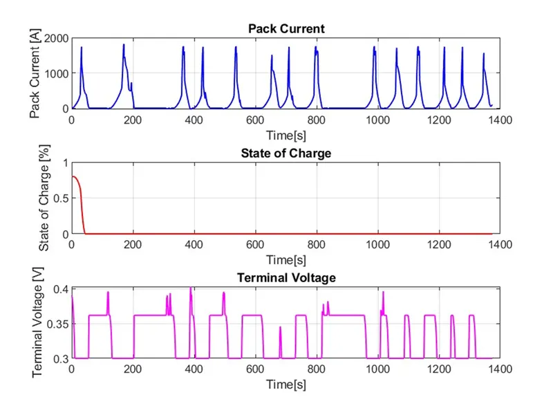
The pack current and voltage fluctuate more in UDDS because of start-stops as the vehicle goes to idle position and battery power is required to start the motor.
This happens once in HWFET at the start as there are no start stops.
Electric Motor Operating Points
UDDS
HWFET