Week 3 - Solving second order ODEs

Solving second order ODEs

Problem statement

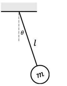
The damped pendulum system is governed by

`(d^2 θ)/(dt^2 )+(b/m) dθ/dt+(g/l) sin⁡θ=0`

Convert second order ODE to first order ODE by assuming

`dθ/dt= θ_1`

And

`(dθ_1)/dt= θ_2`

This implies

`(dθ_2)/dt= (-b/m)θ_1-(g/l)sin⁡〖θ_1 〗`

Input values

Assign input values and initial conditions for displacement and angular velocity as shown below.

Create time array.

%solving second order ode that describes a pendulum mass system

clear all;
clc;
close all;

%inputs

b = 0.05;                     %damping coefficient in Ns/m
m = 1;                     %mass in kg
g = 9.81;                     %acceleration due to gravity in m/s2
l = 1;                       %lenghth of pundulum in m

%initial condition
%diplacement is 0 and velocity is 3rad/s

theta0 = [0;3];
    
%time spaan
%time goes from 0 to 10 seconds with 500 values in between

tspan = linspace(0,20,500);

Function definition

Create function that takes in input variables and solves the equations and stores the values in a matrix

%ode_func definition

function[dtheta_dt] = ode_func(t,theta,b,g,l,m);
theta1 = theta(1);
theta2 = theta(2);
dtheta1_dt = theta2;
dtheta2_dt = -(b/m)*theta2-(g/l)*sin(theta1);
[dtheta_dt] = [dtheta1_dt;dtheta2_dt];
end

ODE solver

Matlab has an inbuilt function for solving ODE’S called ode45

[t result] = ode45(@(t,theta) ode_func(t,theta,b,g,l,m),tspan,theta0);

where tspan integrates the system of differential equations from 0 to 20 with initial conditions theta0. Each row in the solution array result corresponds to a value returned in column vector t.

Plot displacement and angular velocity

%plot

figure(1)
hold on
xlabel('time');
ylabel('plot');
title('plot vs time');
plot(t,result(:,1),'color','r',LineWidth=1);
plot(t,result(:,2),'color','c',LineWidth=1);
hold off


%counter
ct = 1;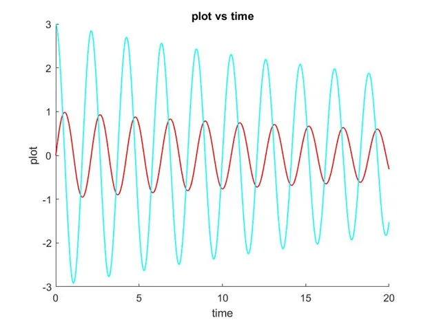

Pendulum animation

Pendulum coordinates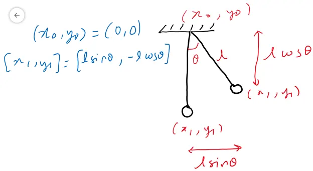

Initialize [x0,y0] = [0,0]

[x1,y1] is calculated for every value of theta which is stored in the first column of result. Hence,

%create pendulum image
for i = 1:length(result);
x0 = 0;
y0 = 0;

x1 =  l*sin(result(i,1));
y1 = -l*cos(result(i,1));

i would go from 1 to 500 and [x1,y1] coordinate will be calculated 500 times.

Plot pendulum string along with mass at the end

String is plotted by providing [x,y] coordinates.

Mass is plotted by marker function ‘-o’ which plots a circle.

Location of the circle is given by ‘markerindices’ followed by the data point at which circle needs to be plotted. In this case the circle is at (x1,y1) which is the second data point.

figure(2)
plot([x0 x1], [y0 y1],'-o','MarkerIndices',2,'MarkerFaceColor','r','color','b');

pause(0.001);
axis([-1 1 -2 0]);

%every single plot is stored in M array using the getframe command
M(ct) = getframe(gcf);
ct=ct+1;
end

%animation
%movie is generated with all frames stored in M
movie(M);             
videofile = VideoWriter('pendulum','Uncompressed AVI');
open(videofile)
writeVideo(videofile,M)
close(videofile)

Animation link

https://www.youtube.com/watch?v=qUOfSXEN6to