Otto Cycle

Otto Cycle

OBJECTIVE

• Write a program to solve the air standard otto cycle in matlab.
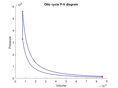
• Plot the P-V diagram.
• Calculate the thermal efficiency of the engine

OTTO CYCLE

An Otto cycle is an idealized thermodynamic cycle that describes the functioning of a SI piston engine.

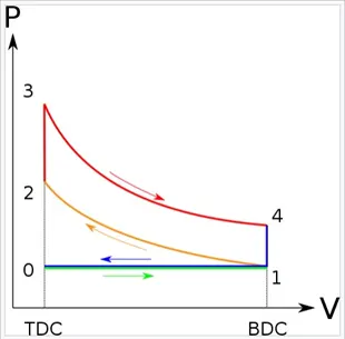
PROCESS

• Process 0–1 a mass of air is drawn into piston/cylinder arrangement at constant pressure.
• Process 1–2 is an adiabatic (isentropic) compression of the charge as the piston moves from bottom dead center(BDC) to top dead center (TDC).
• Process 2–3 is a constant-volume heat transfer while the piston is at top dead center.
• Process 3–4 is an adiabatic (isentropic) expansion (power stroke).
• Process 4–1 completes the cycle by a constant-volume process in which heat is rejected from the air while the piston is at bottom dead center.
• Process 1–0 the mass of air is released to the atmosphere in a constant pressure process.

INPUTS

State variables

P1 = 101325 N/

T1 = 500K

γ = 1.4

T3 = 2300K

Engine parameters

Bore diameter (d)= 0.1
Stroke (l)= 0.1m

Connecting rod = 0.15m

Compression ratio(r) = 12

THEORY

Ideal gas law

`PV/T=CONSTANT`

For isentropic compression,

`P(V^γ)=CONSTANT`

Compression ratio,

r=(Vs + Vc)/(Vc)

Swept volume,

`Vs= (π/4)*d^2*l`

Clearance volume,

`V_c= V_(s )/(r-1)`
then,

state 2 variables

`V_1=V_(s )+ V_c`

`V_2= V_c`

`P_2=P_1*r^γ`

`T_2=P_2*V_2*T_1/(P_1*V_1)`

state 3 variables

`V_3= V_2`

`P_3=P_2*T_3/(T_2)`

state 4 variables

`V_4= V_1`

`P_4=P_3*〖(V_3/V_4)〗^γ`

Writing the program

1. Define all input variables

   %program for olotting the otto cycle
   
   clear all 
   clc
   close all
   
   %input variables
   
   %state variables
   
   p1 = 101325;           %pressure at 1 in N/m2
   t1 = 500 ;              %temperature at 1 in kelvin
   t3 = 2300 ;             %temperature at 3 in kelvin
   gamma = 1.4;
   
   %engine geometric parameters
   
   d = 0.1;                 %bore diameter in m2
   l = 0.1;                 %stroke in m
   r = 12;                  %compression ratio 
   con_rod = 0.15;          %connecting rod
   ​

2. Calculate swept and clearance volume

   %swept and clearance volume
   vs = (pi/4)*d^2*l;
   vc = vs/(r-1);
   v1 = vs + vc;
   v2 = vc;

3. Calculate state variables

   %state 2 variables
   p2 = p1*r^gamma;
   t2 = p2*v2*t1/(p1*v1);
   
   %state 3 variables
   v3 = v2;
   p3 = p2*t3/t2;
   
   
   %state 4 variables
   v4 = v1;
   p4 = p3*((v3/v4)^gamma);

4. Plot all states

   %plot state variables
   
   figure(1);
   hold on;
   plot(v1,p1,'*','color','r');
   plot(v2,p2,'*','color','r');
   plot(v3,p3,'*','color','r');
   plot(v4,p4,'*','color','r');

5. Create function for engine kinematics

   %volume function
   function [V] = engine_kinematics(d,l,con_rod,r,start_crank,end_crank)
   a = l/2;
   R = con_rod/a;
   vs = (pi/4)*d^2*l;
   vc = vs/(r-1);
   
   theta = linspace(start_crank,end_crank,100);
   
   term1 = 0.5*(r-1);
   term2 = R+1-cosd(theta);
   term3 = (R^2-sind(theta).^2).^0.5;
   V = (1+term1*(term2-term3)).*vc;
   
   end​

6. Calculate expansion and compression volumes for various crank angles

   v_compression = engine_kinematics(0.1,0.1,0.15,12,180,0);
   C = p1*v1^gamma;
   p_compression = C./((v_compression).^gamma);
   
   
   
   v_expansion = engine_kinematics(0.1,0.1,0.15,12,0,180);
   C = p3*v3^gamma;
   p_expansion = C./((v_expansion).^gamma);​

7. Calculate efficiency

   Thermal efficiency is give by,

   `η=1-1/(r^((γ-1)))`

8. Plot PV diagram

%join the points with accurate plots
plot(v_compression,p_compression,'color','b','LineWidth',1);
plot(v_expansion,p_expansion,'color','b','LineWidth',1);
plot([v2 v3],[p2 p3],'color','b','LineWidth',1);
plot([v4 v1],[p4 p1],'color','b','LineWidth',1);
xlabel('Volume');
ylabel('Pressure');
title('Otto cycle P-V diagram');

OUTPUT

THERMAL EFFICIENCY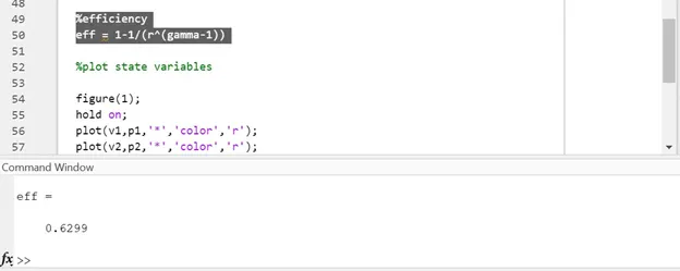

PLOTS