Project 2

Rankine cycle Simulator

Abhishek Patil | 10/04/2022

Objective

• Create a Rankine Cycle Simulator using MATLAB.
• Then, plot the corresponding T-s and h-s plots for the given set of inputs. Title and axes labels are a must, while legends could be used if necessary.

Rankine cycle

The Rankine cycle is an idealized thermodynamic cycle describing the process by which certain heat engines, such as steam turbines or reciprocating steam engines, allow mechanical work to be extracted from a fluid as it moves between a heat source and heat sink. The Rankine cycle is named after William John Macquorn Rankine, a Scottish polymath professor at Glasgow University.

Working

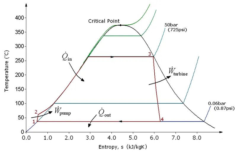
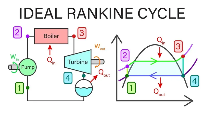
• Process 1–2: The working fluid is pumped from low to high pressure. As the fluid is a liquid at this stage, the pump requires little input energy. Process 1-2 is isentropic compression.
• Process 2–3: The high-pressure liquid enters a boiler, where it is heated at constant pressure by an external heat source to become a dry saturated vapour. The input energy required can be easily calculated graphically, using an enthalpy–entropy chart (h–s chart, or Mollier diagram), or numerically, using steam tables or software. Process 2-3 is constant pressure heat addition in boiler.
• Process 3–4: The dry saturated vapour expands through a turbine, generating power. This decreases the temperature and pressure of the vapour, and some condensation may occur. The output in this process can be easily calculated using the chart or tables noted above. Process 3-4 is isentropic expansion.
• Process 4–1: The wet vapour then enters a condenser, where it is condensed at a constant pressure to become a saturated liquid. Process 4-1 is constant pressure heat rejection in condenser.

MATLAB Script

% rankine cycle simulator

 

clc;

clear all;

close all;

 

% title info

 

disp('Rankine Cycle ');

 

% input

 

P1 = input('Pressure (bar) at turbine inlet = ');

T1 = input('Temperature (degrees Celsius) at turbine inlet = ');

P2 = input('Pressure (bar) at condenser inlet = ');

 

% data extraction

 

% state 1

 

H1 = XSteam('h_pT',P1,T1);       % enthalpy at state 1

S1 = XSteam('s_pT',P1,T1);       % entropy at state 1

 

% state 2

 

S2 = S1;                         % isentropic expansion

Sf2 = XSteam('sL_p',P2);         % saturated liquid entropy

Sg2 = XSteam('sV_p',P2);         % saturated vapour entropy

X2 = (S2-Sf2)/(Sg2-Sf2);         % vapour fraction

Hf2 = XSteam('hL_p',P2);         % saturated liquid enthalpy

Hg2 = XSteam('hV_p',P2);         % saturated vapour enthalpy

H2 = Hf2 +(X2*(Hg2-Hf2));        % enthalpy at state 2

 

% state 3

 

P3 = P2 ;                        % constant pressure heat rejection

S3 = XSteam('sL_T',P3);          % entropy at state 3

H3 = XSteam('hL_T',P3);          % enthalpy at state 3

 

% state 4

 

S4 = S3;                         % entropy at state 4

P4 = P1;                         % pressure at state 4

 

% work done by turbine

 

Wt = H1-H2;                      % KJ/Kg

 

% pump work

 

v3 = XSteam('vL_T',P3);          % Specific volume (m3/kg)

Wp = v3*(P4-P3)*100;             % KJ/Kg

H4 = H3 + Wp;                    % Enthalpy at state 4    (kJ/kg)

 

% net work

 

Wnet = Wt- Wp;                  % KJ/Kg

 

% back work raio

 

back_work_ratio = Wp/Wt;      

 

% heat in the system

 

Qin = H1-H4;                    % KJ/Kg

 

 

% heat out of the system

 

Qout = H2-H3;                   % KJ/Kg

 

% thermal efficiency

 

eff = (Wnet/Qin)*100;

 

% specific steam consumption

 

ssc = 3600/Wnet;               % mass flow rate = 3600

 

% state point temperatures

 

T3 = XSteam('Tsat_p',P3);

T2 = T3;

Cp4 = XSteam('Cp_ps',P4,S4);

Cv4 = XSteam('Cv_ps',P4,S4);

k = Cp4/Cv4;

T4 = T3/((P3/P4)^((k-1)/k));

 

% vapour and liquid line parameter

 

T6 = XSteam('Tsat_p',P1);

S5 = XSteam('sL_p',P1);

S6 = XSteam('sV_p',P1);

H5 = XSteam('hL_p',P1);

H6 = XSteam('hV_p',P1);

T5 = T6;

 

% saturation curve plot

 

T = linspace(1,375,1000);

for i =1:length(T)

 

    Sf(i) = XSteam('sL_T',T(i));            %Saturated liquid entropy

    Sg(i) = XSteam('sV_T',T(i));            %Saturated vapour entropy

    Hf(i) = XSteam('hL_T',T(i));            %Saturated liquid enthalpy

    Hg(i) = XSteam('hV_T',T(i));            %Saturated vapour enthalpy

end

 

% plotting T-S graph

 

figure(1);

hold on;

plot(Sf,T,'color','r','LineWidth',2);

plot(Sg,T,'color','r','LineWidth',2);

plot([S1 S2],[T1 T2],'color','k','LineWidth',2);

plot([S2 S3],[T2 T3],'color','k','LineWidth',2);

plot([S3 S4],[T3 T4],'color','k','LineWidth',2);

plot([S4 S5],[T4 T5],'color','k','LineWidth',2);

plot([S5 S6],[T5 T6],'color','k','LineWidth',2);

Sc1 = linspace(S6,S1,1000);

 

for j = 1:length(Sc1)

  

    Tc1(j) = XSteam('T_ps',P1,Sc1(j));

end

 

plot(Sc1,Tc1,'color','k','LineWidth',2);

text(S1+0.1,T1,'1');

text(S2+0.1,T2,'2');

text(S3,T3-20,'3');

text(S4,T4+20,'4');

title('Entropy Vs Temperature')

xlabel('Entropy [Kj/Kg-K]')

ylabel('Temperature [degrees C]')

legend('Saturation Curve')

axis([-1 10 -100 450]);

 

 

% plotting H-S graph

 

figure(2);

hold on;

plot(Sf,Hf,'color','r','LineWidth',2);

plot(Sg,Hg,'color','r','LineWidth',2);

plot([S1 S2],[H1 H2],'color','k','LineWidth',2);

plot([S2 S3],[H2 H3],'color','k','LineWidth',2);

plot([S3 S4],[H3 H4],'color','k','LineWidth',2);

 

Hc = linspace(H4,H5,100);

 

for k = 1:length(Hc)

  

    Sc2(k) = XSteam('s_ph',P1,Hc(k));

end

 

plot(Sc2,Hc,'color','k','LineWidth',2);

plot([S5 S6],[H5 H6],'color','k','LineWidth',2);

 

for l = 1:length(Sc1)

 

    Hc1(l) = XSteam('h_ps',P1,Sc1(l));

end

  

plot(Sc1,Hc1,'color','k','LineWidth',2);

 

text(S1+0.1,H1,'1');

text(S2+0.1,H2,'2');

text(S3,H3-100,'3');

text(S4,H4+201,'4');

title('Entropy Vs Entropy')

xlabel('Entropy [Kj/Kg-K]')

ylabel('Enthalpy [Kj/Kg]')

axis([-1 10 -200 3500]);

 

% results

 

disp('Results');

 

fprintf('\nState 1\n\n')

fprintf('P1 = %f bar\n',P1);

fprintf('T1 = %f degrees C\n',T1);

fprintf('H1 = %f Kj/Kg\n',H1);

fprintf('S1 = %f Kj/Kg-K\n\n',S1);

 

fprintf('State 2\n\n')

fprintf('P2 = %f bar\n',P2);

fprintf('T2 = %f degrees C\n',T2);

fprintf('H2 = %f Kj/Kg\n',H2);

fprintf('S2 = %f Kj/Kg-K\n',S2);

fprintf('X2 = %f \n\n',X2);

 

fprintf('State 3\n\n')

fprintf('P3 = %f bar\n',P3);

fprintf('T3 = %f degrees C\n',T3);

fprintf('H3 = %f Kj/Kg\n',H3);

fprintf('S3 = %f Kj/Kg-K\n\n',S3);

 

fprintf('State 4\n\n')

fprintf('P4 = %f bar\n',P4);

fprintf('T4 = %f degrees C\n',T4);

fprintf('H4 = %f Kj/Kg\n',H4);

fprintf('S4 = %f Kj/Kg-K\n\n',S4);

 

fprintf('Turbine Work = %f Kj/Kg\n',Wt);

fprintf('Pump Work = %f Kj/Kg\n',Wp);

fprintf('Net Work = %f Kj/Kg\n',Wnet);

fprintf('Efficiency = %f \n',eff);

fprintf('SSC = %f Kj/KWh\n',ssc);

fprintf('Back work ratio = %f \n',back_work_ratio);

 

Explanation

• XSteam data is used to extract the entropy, enthalpy values at pressure and temperature values for saturated liquid and vapor conditions.
• The following inputs were taken from the problem statement
• Turbine Inlet temperature = 400° C

Turbine Inlet Pressure = 30 bars

Turbine Outlet Pressure = 0.05 bars = Condenser Inlet Pressure

• Pump work, turbine work is calculated from enthalpy values.
• Net work is the difference between them
• Heat in , heat out, efficiency and specific steam consumption is calculated.
• Temperature, entropy and enthalpy values are extracted from XSteam at liquid and vapour lines for plotting the curve beyond point 4.

Results

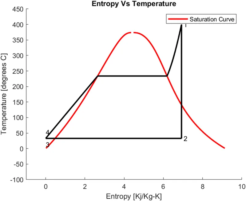
Temperature entropy curve

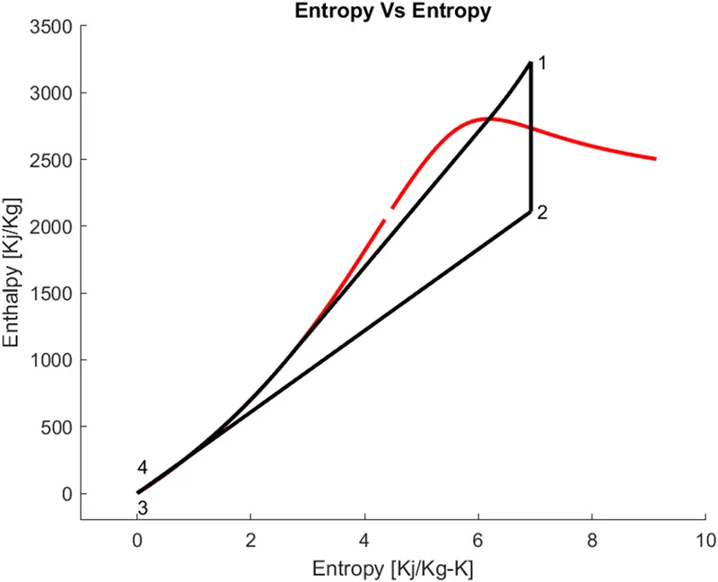
Enthalpy entropy curve

Command window results

Rankine Cycle

Pressure (bar) at turbine inlet = 30

Temperature (degrees Celsius) at turbine inlet = 400

Pressure (bar) at condenser inlet = 0.05

Results

State 1

P1 = 30.000000 bar

T1 = 400.000000 degrees C

H1 = 3231.571027 Kj/Kg

S1 = 6.923259 Kj/Kg-K

State 2

P2 = 0.050000 bar

T2 = 32.875490 degrees C

H2 = 2110.708212 Kj/Kg

S2 = 6.923259 Kj/Kg-K

X2 = 0.814256

State 3

P3 = 0.050000 bar

T3 = 32.875490 degrees C

H3 = 0.169407 Kj/Kg

S3 = 0.000618 Kj/Kg-K

State 4

P4 = 30.000000 bar

T4 = 32.960591 degrees C

H4 = 3.165016 Kj/Kg

S4 = 0.000618 Kj/Kg-K

Turbine Work = 1120.862815 Kj/Kg

Pump Work = 2.995610 Kj/Kg

Net Work = 1117.867205 Kj/Kg

Efficiency = 34.625980

SSC = 3.220418 Kj/KWh

Back work ratio = 0.002673

>>