Project 1
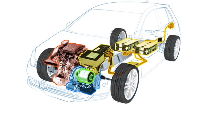
Project 1
forward energy-based fuel consumption model of a conventional vehicle.
Abhishek Patil | 07/03/2022
Objective
To compute the fuel economy numbers for the given vehicle (kmpl) on the urban cycle (UDDS) and highway cycle (HWFET). Also, to analyze and understand the vehicle operating
points in terms of engine speed, torque, transmission speeds, pedal positions, gear, distance traveled, etc.
- Tabulate the fuel economy numbers (kmpl) for UDDS and HWFET cycle. This forms the baseline numbers for comparing with the future hybrid version
- Plot the time trace for engine, transmission input, transmission output and wheel speed on one plot.
- Plot engine torque, engine power, fuel rate and fuel consumption using subplots.
- Plot accelerator and brake pedal, gear command, vehicle desired and actual speed, vehicle distance using subplots.
- Plot the engine operating points on the engine fuel map.
- Write down appropriate brief comments on each of these plots, describing the vehicle behavior throughout the drive cycle.
- Generate the plots for both drive cycle
Forward Modelling
In this type of modeling, you have a specific model that defines the "current" state of your system.
Forward modeling is the use of a model in order to simulate an outcome. The problem of getting the model to produce data from the input is called the forward problem.
The forward model takes certain parameters and produces data that can then be compared with the actual observations.
The opposite procedure is called the inverse problem
Initialization script
This is a MATLAB script used to load all the variables required for running the Simulink model and for post-processing.
%%%%%%%%%%%%%%%%%%%%%%%%%%%%%%%%%%%%%%%%%%%%%%%%%%%%%%%%%%%%%%%%%%%%%

%% Skill-Lync -> Hybrid Drives Development

% Project 1 - Conventional Vehicle Model

% By - Ullekh Gambhira


% Description:


%% Initialization File

% Initialization file for loading the variables for the Conventional vehicle simulation model


%% Vehicle Parameters

M = 1500;       % Vehicle weight [kg]

Cr = 0.015;     % Rolling resistance coefficient

Rw = 0.35;      % Rolling radius [m]

Cd = 0.33;      % Drag coefficient

Af = 2;         % Frontal area [m2]

rhoa = 1.225;   % Air density [kg/m3]

Vwind = 0;      % Wind velocity [kmph]

g = 9.81;       % Gravitational acceleration [m/s2]

theta = 0;      % Slope [deg]

myu_road_tire = 1; % Coefficient of friction between tire - road interface


%% Powertrain Parameters

FDR = 3.73;                         % Final Drive Ratio / Diff Ratio

DiffEff = 0.99;                     % Differential efficiency (assumed independent of operating conditions)


NumGear = 4;                        % Number of gears in transmission

TransGear = [1:NumGear];            % Transmission Gears

TransRatio = [3.06, 1.62, 1, 0.7];  % Corresponding Transmission ratios

TransEff = 0.90;                    % Transmission efficiency (assumed independent of operating conditions)


TC_SR = [0, .5, .6, .7, .8, .87, .92, .94, .96, .97, 1];   % Torque Converter Speed Ratio (Matlab default) -> TurbSpd/PumpSpd

TC_TR = [2.232, 1.5462, 1.4058, 1.2746, 1.1528, 1.0732, 1.0192, 1, 1, 1, 1];   % Torque Converter Torque Ratio (Matlab default) -> TurbTrq/PumpTrq

TC_Cf = 1e-4 * [.72558, .66322, .63463, .59042, .51331, .4144, .29287, .22444, .12186, .04386, 0]; % Torque Converter Capacity Factor (Matlab default) -> PumpTrq/PumpSpd^2 [Nm/rpm^2]


load Vehicle_Data/Engine_data_1_9L_Saturn_95kW

load Vehicle_Data/Trans_Shift_map


%% Driver Parameters

Kp = 10;                    % P gain for driver PI model

Ki = 1;                     % I gain for driver PI model

Drive_Cycle_Select = 1;     % Drive cycle selection


% Drive cycle values in m/s


if Drive_Cycle_Select == 1

    load DriveCycles/UDDS;


elseif Drive_Cycle_Select == 2

    load DriveCycles/HWFET;


elseif Drive_Cycle_Select == 3

    load DriveCycles/FTP;


elseif Drive_Cycle_Select == 4

    load DriveCycles/US06;


elseif Drive_Cycle_Select == 5

    load DriveCycles/NEDC;


elseif Drive_Cycle_Select == 6

    load DriveCycles/WLTP;


end


time_end = cyc_time(end);

vel_end = cyc_vel(end);
Simulink Model
In this project, a typical midsize car with a 1.9L engine and a 4-speed automatic transmission is considered. Data is taken from ADVISOR data base developed by NREL, USA. Transmission shift map and controller is taken from Matlab/Simulink example database.
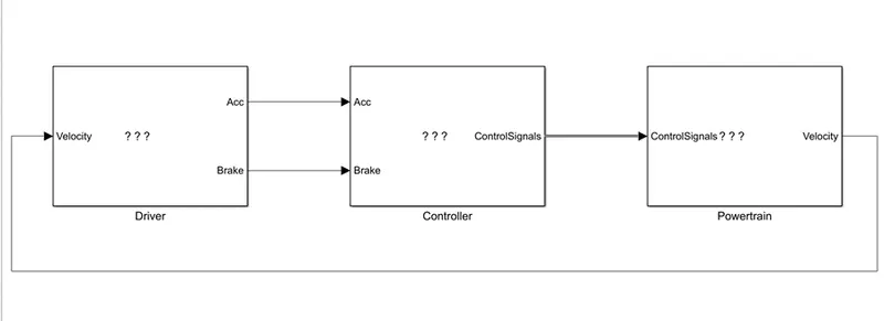
Driver model
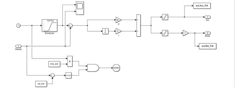
It is modeled using a ‘Driver’ block, which is a basic PI controller that generates accelerator and brake pedal outputs to match the desired
and actual vehicle speeds.
It compares the actual velocity and the drive cycle velocity and calculates the difference. Depending on whether the difference is positive or negative, it informs the driver whether to accelerate or brake.
Control model
The ‘Controller’ block is the brains of the vehicle, representing the electronic controls units. Based on the driver inputs, it generates desired engine torque, desired transmission gear and desired brake torque. These inputs are fed to the ‘Powertrain’ block which represents the drivetrain of the vehicle.
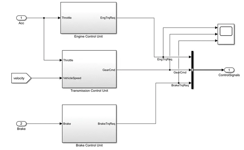
It consists of the following sub systems
- Engine Control Unit
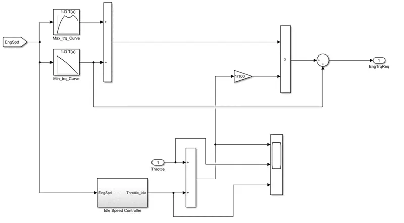
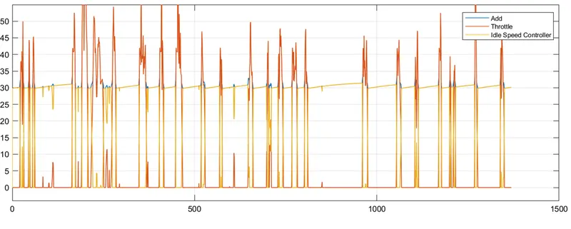
The idle speed controller keep the speed above the idle speed and make sure that the engine is idling
The accelerator pedal from the driver unit provides the throttle signal as an input.
It has two look up tables for maximum and minimum torque curves for various speed values.
The input to the tables is the engine speed. This input along with the throttle and idle speed controller signals are multiplied together to get the required engine torque.
Engine control unit output
- Transmission Control Unit
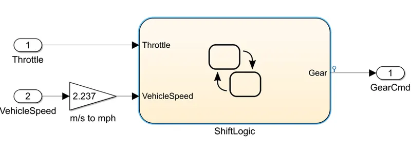
It uses state flow to determine gear shifting.
Velocity and throttle is taken as inputs and the gear used currently is given as an output
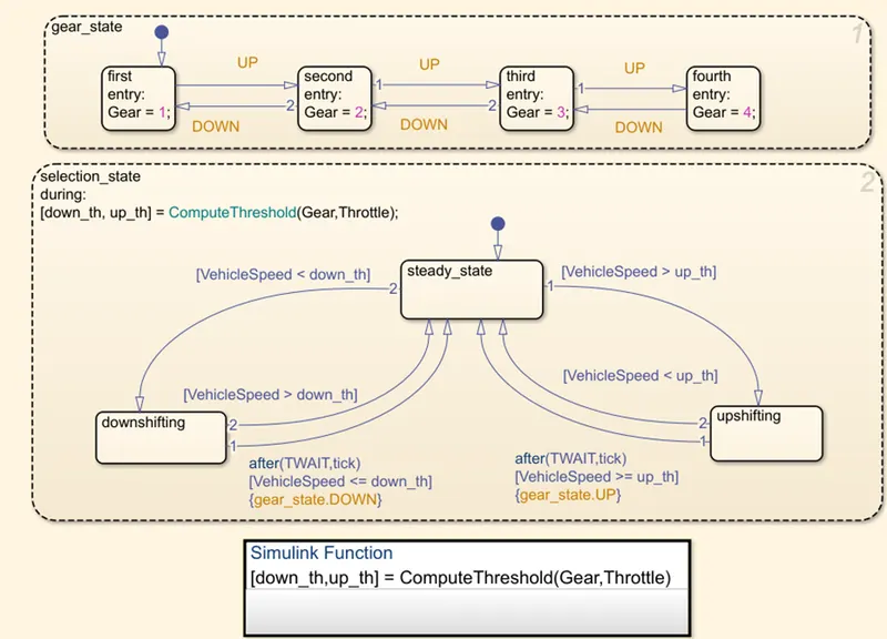
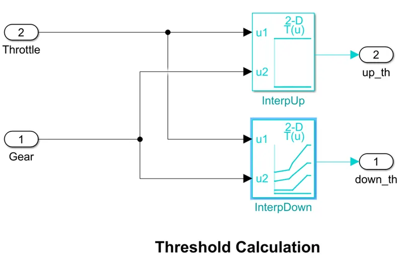
The Gear_state state block decides which gear to shift to using the UP and DOWN decision arrows.
The decision is done by the selection_state state block. Using the ComputeThreshold Simulink function it calculates the values of up_th and down_th which decide whether the gear state should be up or down.
- Brake Control Unit
The brake torque is calculated analytically and multiplying it with the brake signal, the magnitude of the brake torque which is required is generated.
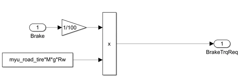
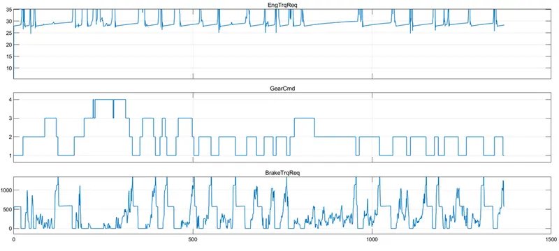
The above three signals are connected to a bus, which is transferred to the powertrain block
The three signals are shown below.
Powertrain Model
Every component of the system that converts power into movement is included in the power train block.
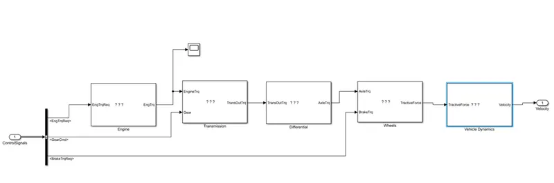
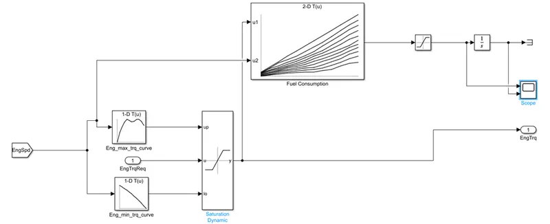
- Engine
Map based model is used to model the fuel consumption of the engine.
The max and min torque curves act as upper and lower bounds for the engine torque signal which is given to the 2D look up table of fuel consumption. The look up table gives the fuel flow rate and the integrator gives the total fuel consumed until that point.
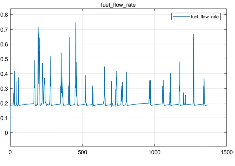
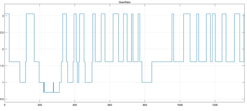
- Transmission
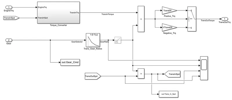
The engine torque and the transmission speed go into the torque converter.
The gear output signals are sent to the transmission gear ratio look up table.
The gear ratio is then multiplied with the transmission torque and transmission efficiency to get the transmission output torque.
The gear ratio is also multiplied with the transmission speed to get the transmission output speed.
- Differential
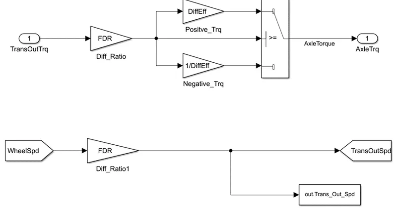
The wheel speed is multiplied by the differential ratio to get the output speed
Transmission torque is further multiplied or divided by the differential efficiency depending on whether the torque is positive or negative respectively.
The output is the axle torque.
- Wheels
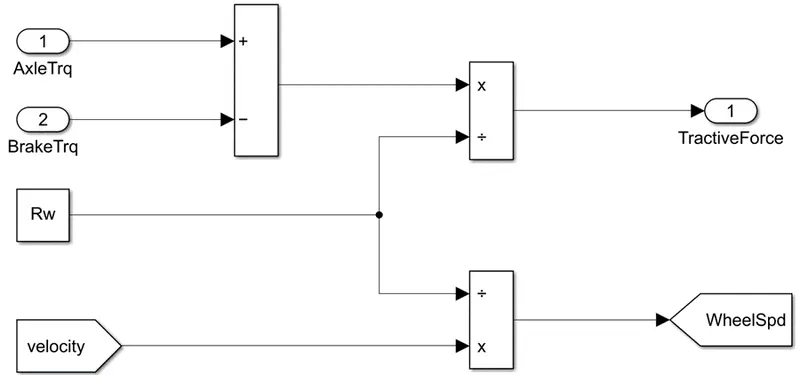
The brake torque is subtracted from the axle torque to get the net torque, which is then divided by the wheel radius to get the tractive force.
The velocity is divided by the wheel radius to get wheel speed.
- Vehicle Dynamics
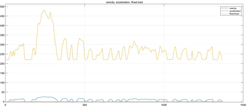
The dynamic equation for calculating the road load is
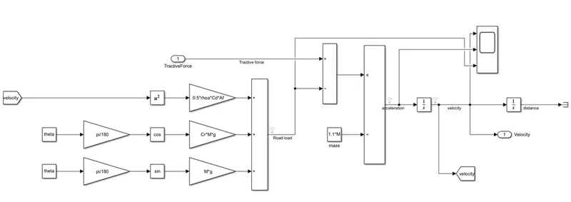
This equation is represented using the various mathematical blocks, which after integrating gives us the velocity

MATLAB code for post processing
%%%%%%%%%%%%%%%%%%%%%%%%%%%%%%%%%%%%%%%%%%%%%%%%%%%%%%%%%%%%%%%%%%%%%

%% Skill-Lync -> Hybrid Drives Development

% Project 1 - Conventional Vehicle Model

% By - Ullekh Gambhira


% Description:

% The following file is to used with the Initialization file and Simulink

% results for post-processing of the data.

% The file is incomplete, has some examples of how the data is imported

% into a readable format, data analysis and plotting examples.

% Based on the project task, use commands in a similar format as given

% below, to analyse the data and generate required plots.

% You can change variable names if desired


%% Post-Processing File

%  File for post-processing the Conventional vehicle simulation model data


%% Renaming variables


clc;


Time = out.tout;

Acc_Pdl = out.Acc_Pdl;          % Accelerator pedal [%]

Brk_Pdl = out.Brk_Pdl;          % Brake pedal [%]

Gear_Cmd = out.Gear_Cmd;        % Transmission gear

Trans_In_Spd = out.Trans_In_Spd*30/pi;  % Transmission input speed [rpm]

Trans_Out_Spd = out.Trans_Out_Spd*30/pi;% Transmission output speed [rpm]

Eng_Trq = out.EngTrq.Data(:,1);          % Engine brake torque [Nm]

Eng_Fuel_Consump = out.totalfuel.Data(:,1);    % Engine fuel consumption [g]

Veh_Dist = out.VehDist.Data(:,1)/1000;   % Distance traveled by vehicle [km]

Veh_Spd = out.VehSpd.Data(:,1)*(18/5);     % Vehicle speed [kmph]

Eng_Fuel_rate = out.fuelflowrate.Data(:,1);  % Engine Fuel Rate %

Wheel_Spd = out.WheelSpd.Data(:,1)*30/pi;          % Wheel Speed


% vehicle characteristics

Eng_spd = out.EngSpd.Data(:,1); % Engine Speed m/s

Eng_Spd_rpm = Eng_spd*30/pi;    % engine Speed Rpm


%% Data Analysis

Eng_Pwr = Eng_spd.*Eng_Trq.*((pi/30)/1000);   % Engine brake power [kW]

rho_petrol = 0.7197;                    % Density of petrol [kg/L]

kmpl = Veh_Dist(end)/(Eng_Fuel_Consump(end)/1000/rho_petrol);    % Fuel economy [kmpl]

fprintf('fuel comsumption [Kmpl] = %f',kmpl);


%% Plotting vehicle characteristics time trace

figure('Name','transmission IN/OUT speed')

hold on

plot(Time, Trans_In_Spd, 'linewidth', 1, 'Color', 'black');

plot(Time, Trans_Out_Spd, 'linewidth', 1, 'Color', 'red');

plot(Time, Wheel_Spd, 'linewidth', 1, 'Color', 'green');

plot(Time, Eng_Spd_rpm, 'linewidth', 1, 'Color', 'blue');

ylabel('Speed [rpm]')

xlim([0, Time(end)]);

ylim([0, 5000]);

legend('Trans Input','Trans Output','Wheel Speed','Engine Speed');


%% Plotting Engine charactesticks

figure('Name','Engine charactesticks');

subplot(2,2,1);

plot(Time, Eng_Trq, 'linewidth', 1, 'Color', 'black');

xlabel('Time [s]');

ylabel('Engine Torque (Nm)');

legend('Engine Torque');

grid on;


subplot(2,2,2);

plot(Time, Eng_Pwr, 'linewidth', 1, 'Color', 'blue');

xlabel('Time [s]');

ylabel('Engine Power (kW)');

legend('Engine Power');

grid on;


subplot(2,2,3);

plot(Time, Eng_Fuel_rate, 'linewidth', 1, 'Color', 'red');

xlabel('Time [s]');

ylabel('Engine Fuel Rate (%)');

legend('Engine Fuel Rate');


subplot(2,2,4);

plot(Time, Eng_Fuel_Consump, 'linewidth', 1, 'Color', 'green');

xlabel('Time [s]');

ylabel('Engine Fuel Consumption');

legend('Engine Fuel Consumption');


%% Plotting Fuel Economy Vs Fuel Consumption

figure('Name','Fuel Economy Vs Fuel Consumption');

plot(Eng_Fuel_Consump, Eng_Fuel_rate, 'linewidth', 1, 'Color', 'r');

xlabel('Engine Fuel Consumption');

ylabel('Engine Fuel Rate');

grid on;


%% Plotting Accelerator brake pedals and gear CMD

figure('Name','Accelerator,brake,gear');

subplot(2,1,1);

hold on;

plot(Time, Acc_Pdl, 'linewidth', 1, 'Color', 'black');

plot(Time, Brk_Pdl, 'linewidth', 1, 'Color', 'blue');

xlabel('Time [s]');

ylabel('Pedal(%)');

legend('Accelearator vs Brake pedal');

grid on;


subplot(2,1,2);

plot(Time, Gear_Cmd, 'linewidth', 1, 'Color', 'blue');

xlabel('Time [s]');

ylabel('Gear CMD');

legend('Gear CMD');

grid on;


%% Plotting Gear CMD wrt speed and distance

figure('Name','Gear command wrt Vehicle speed and distance');

subplot(2,1,1);


plot(Veh_Spd, Gear_Cmd, 'linewidth', 1, 'Color', 'blue');

xlabel('vehicle speed (m/s)');

ylabel('Gear CMD');

title('Vehicle Speed vs gear CMD');

grid on;


subplot(2,1,2);

plot(Veh_Dist, Gear_Cmd, 'linewidth', 1, 'Color', 'green');

xlabel('Vehicle Distance');

ylabel('Gear CMD');

title('Vehicle Distance vs gear CMD');

grid on;


%% Plotting engine operating points on engine fuel map

figure('Name','Engine Operating Points');

hold on

grid on

title('Engine Operating Points','fontsize',12);

p1=plot(Eng_map_spd*30/pi,Eng_max_trq,'linewidth',2,'color','r');

p2=line([Eng_map_spd(end)*30/pi Eng_map_spd(end)*30/pi],[0 Eng_max_trq(end)]);

set(p2,'linewidth',1,'linestyle','--','color','k');

p3=line([Eng_map_spd(1)*30/pi Eng_map_spd(1)*30/pi],[0 Eng_max_trq(1)]);

set(p3,'linewidth',1,'linestyle','--','color','k');

[c,h] = contour(Eng_map_spd'*30/pi,Eng_map_trq,Eng_fuel_map');

clabel(c,h);

xlabel('Engine Speed [rpm]');

ylabel('Engine Torque [Nm]');

title('Engine Fuel Consumption Map [g/s]');

axis([Eng_map_spd(1)*30/pi Eng_map_spd(end)*30/pi 0 Eng_map_trq(end)]);
Results
UDDS Cycle
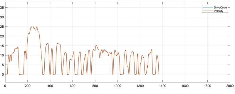
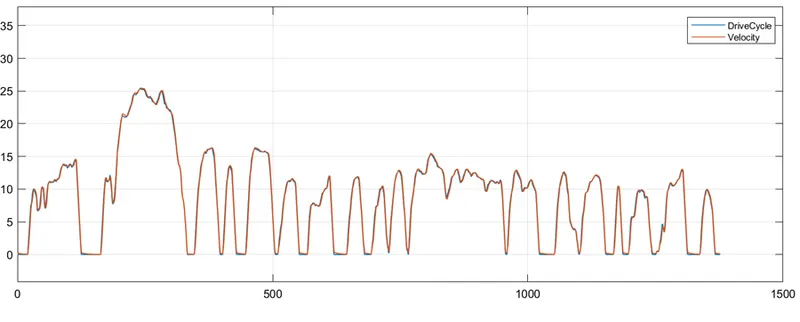
Drive cycle
Fuel consumption (KMPL)

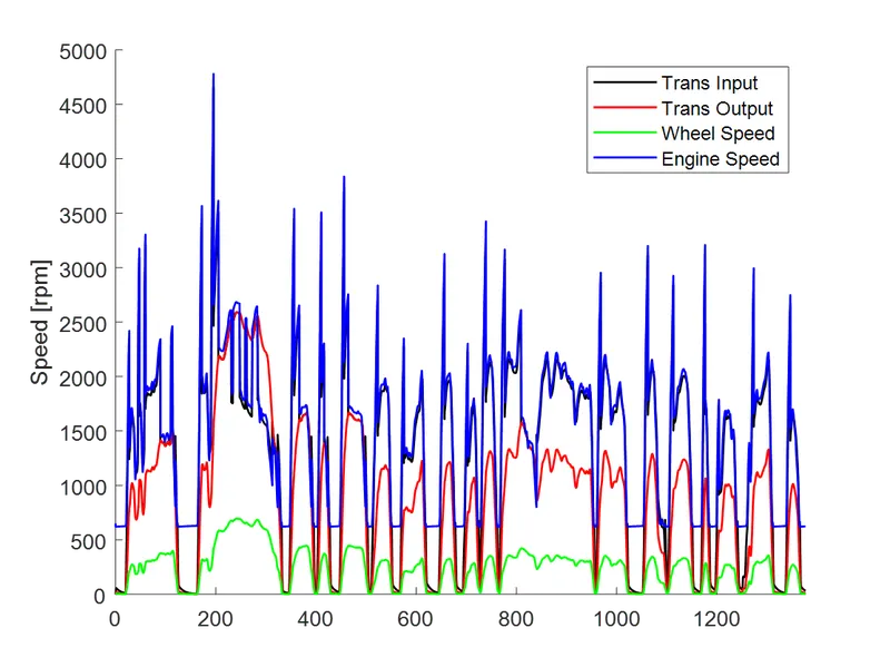
Transmissions speeds, Engine speeds, Wheel speeds
The Engine speed reflects the drive cycle requirements
Transmission speed are less in magnitude because of transmission losses which are represented by transmission efficiency in the code
Due to differential ratio and differential losses the wheel speed is significantly less than transmission speeds
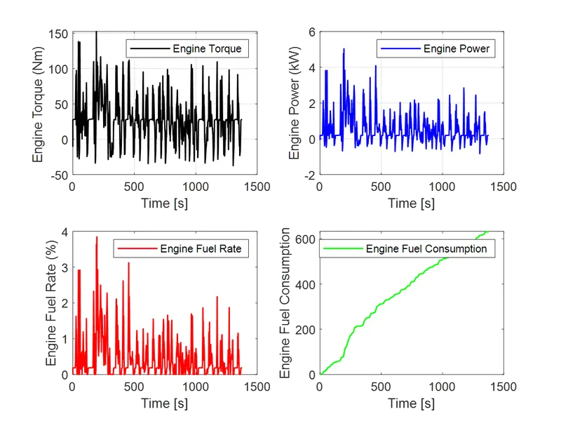
Engine Characteristics
The engine torque and power reflect the drive cycle requirements.
The spikes indicate increase in speeds and the falls indicate the decrease in speeds.
The engine fuel consumption increases with time as the vehicle continues to move.
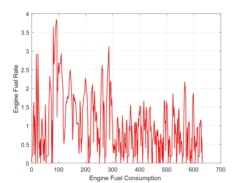
Fuel economy vs Fuel Consumption
The spikes indicate the acceleration points
The falls indicate the brake points
the constant lines indicate areas where the velocity does not vary too much.
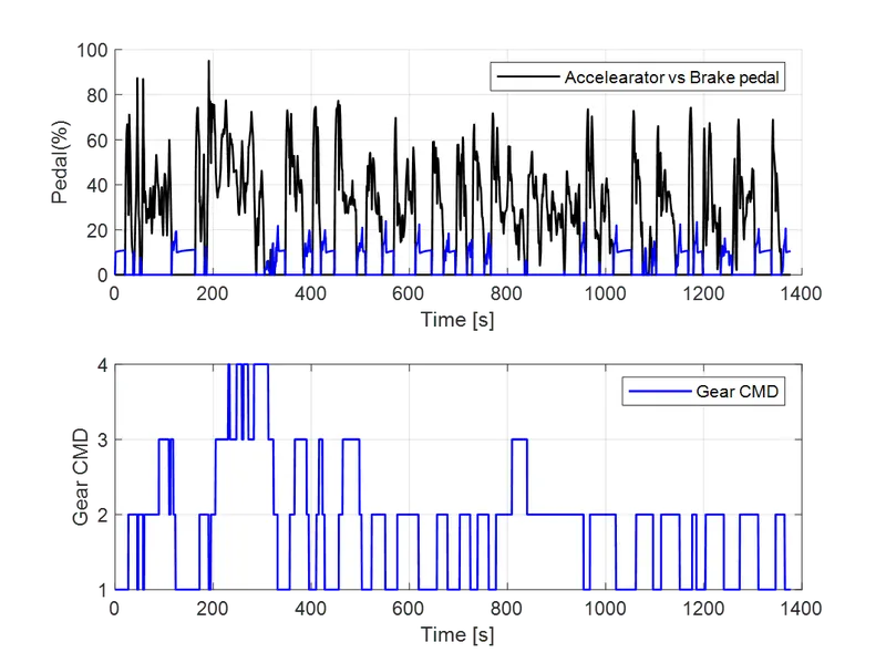
Pedals and gears
The acceleration is mere as compared to the brake instances as seen below.
This implies that the brake torque applied is low.
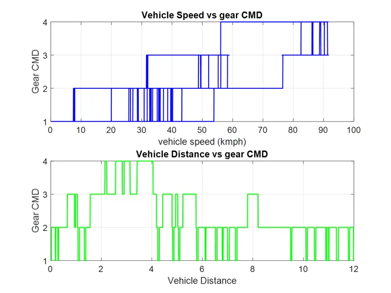
Correspondingly the gear shifting has been displayed below
Gear CMD wrt vehicle Speed and Distance
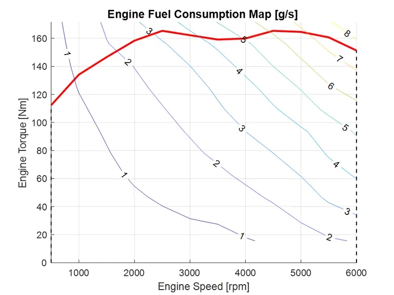
Engine operating points
The max torque curve is indicated in red
HWFET Cycle
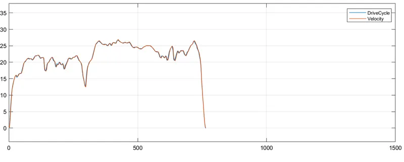
Drive cycle
Fuel consumption (KMPL)
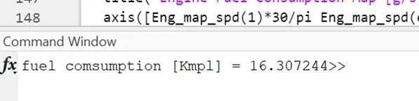
As the fuel consumption is more than UDDS cycle, we can say that HFWET is less economical than UDDS.
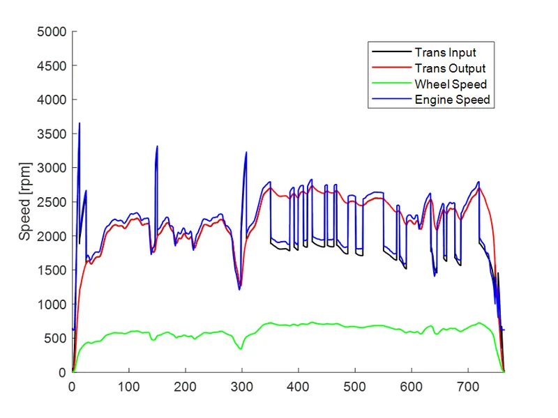
Transmissions speeds, Engine speeds, Wheel speeds
The Engine speed reflects the drive cycle requirements
Transmission speed are less in magnitude because of transmission losses which are represented by transmission efficiency in the code
Due to differential ratio and differential losses the wheel speed is significantly less than transmission speeds
The speed never goes to zero in the cycle which creates a smooth curve as compared to UDDS
Engine Characteristics
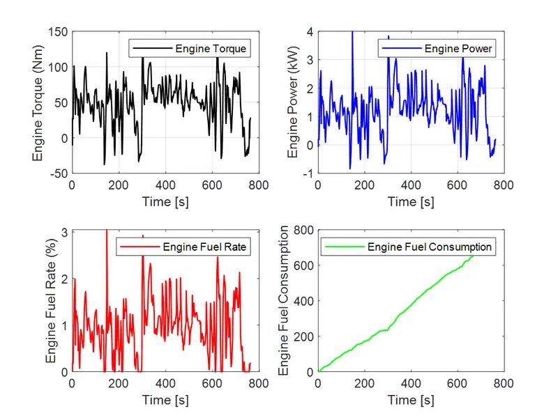
The engine torque and power reflect the drive cycle requirements. They rarely go below zero as the brakes aren’t applied as frequently.
The spikes indicate increase in speeds and the falls indicate the decrease in speeds.
The engine fuel consumption increases with time as the vehicle continues to move.
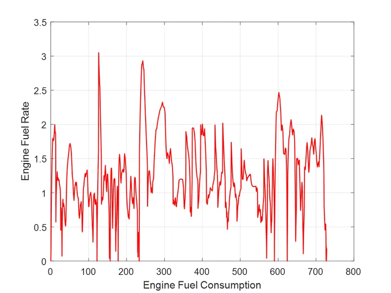
Fuel economy vs Fuel Consumption
The spikes indicate the acceleration points
The falls indicate the brake points which are less than UDDS cycle.
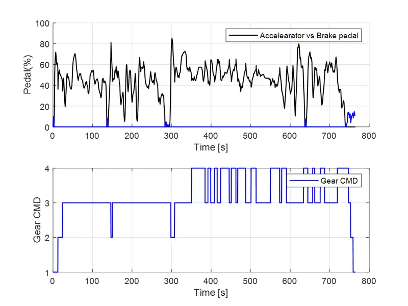
Pedals and gears
The acceleration is more as compared to the brake instances as seen below.
This implies that the brake torque applied is low. Even lower than UDDS cycle
Correspondingly the gear shifting has been displayed below.
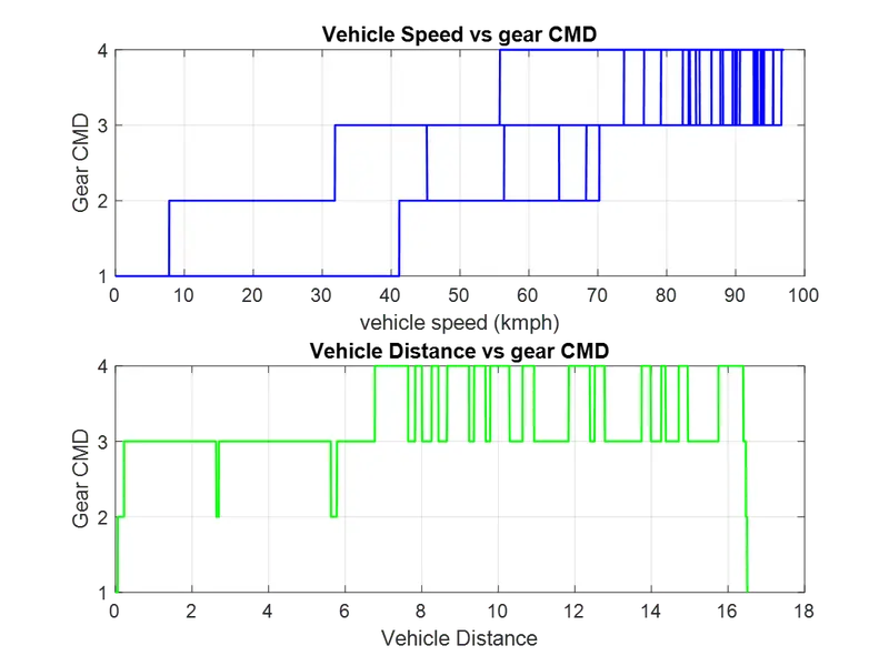
The gears never go to the first gear in the entire cycle.
Gear CMD wrt vehicle Speed and Distance
Engine operating points
The max torque curve is indicated in red