Modelling an electric Car with Li-ion battery

• 1) Aim
• Create a MATLAB model of an electric car that uses a lithium-ion battery and a suitable motor. Choose suitable blocks from Simscape or Powertrain block set. Implement the vehicle speed control using a PID controller and generate brake and accelerator commands.
• 2) Theory, Formulas, and Subsystems and Final Model:
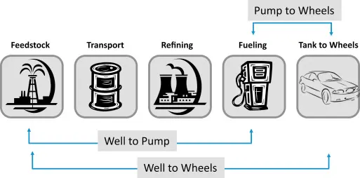
• Advantage of an EV over a conventional ICE by well to wheel analysis:
• A well-to-wheels (WTW) analysis of a vehicle/fuel system covers all stages of the fuel cycle, from energy feedstock recovery (well) to energy delivery at the vehicle’s wheels.
• 
• The calorific value of a fuel is the quantity of heat produced by its combustion – at constant pressure and under “normal” (standard) conditions (i.e. to 0^oC and under a pressure of 1,013 bar).
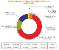
• An electric vehicle can never be called a zero-emission vehicle as the power to charge an EV can come from the burning of fossil fuel especially in India. Below is an image that justifies the claim
• 
• The vehicles used for comparison are TATA NEXON(ICE) and TATA NEXON EV.
  

  TATA NEXON(ICE)	TATA NEXON EV
  Range = 17 Km/L	Range=300 Km/Charge
  Petrol calorific value = 9528 Wh/L	Battery power=30200 Wh
  Average energy consumed at wheel : Tank to wheel Petrol calorific value/Range=560.47 Wh/Km	Average energy consumed at wheel : Tank to wheel =Battery power/range=100.66 Wh/Km
  Refinement and transportation of fuel=67%	Charging and discharging efficiency= 80%
  Average energy with production and transmission losses = well to wheel =Average energy with wheel/efficiency = 836.52 Wh/Km	Average Energy with Battery losses=Averageenergy/Efficiency = 125.83Wh/km Production and transmission efficiency of electricity=30% Average energy at wheel considering all efficiencies Well to wheel = 419.44 Wh/km

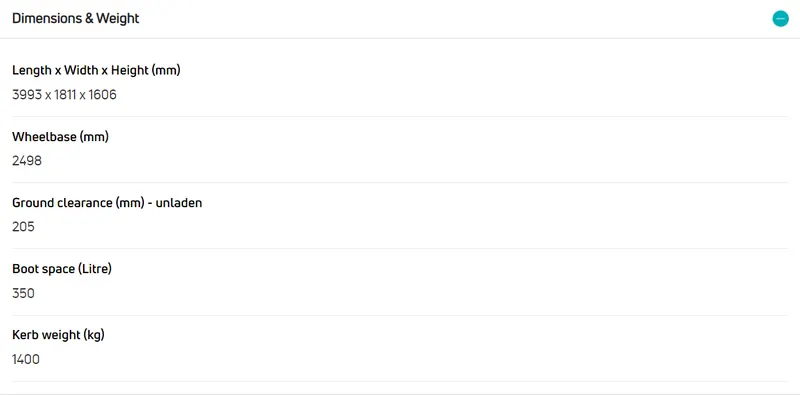
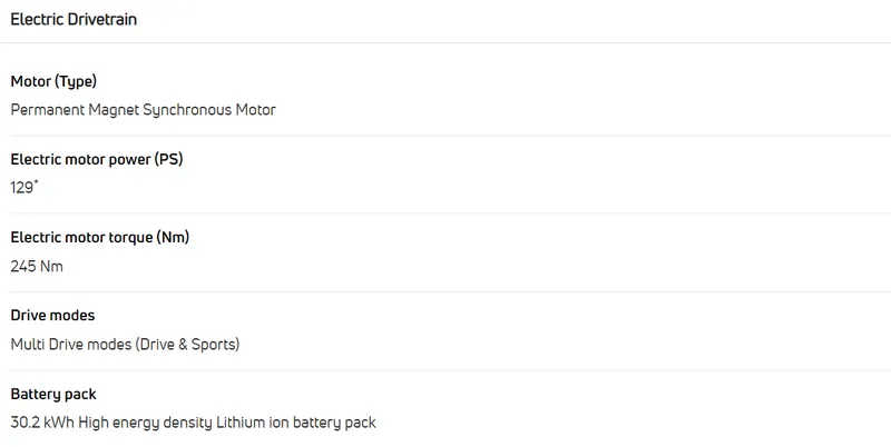
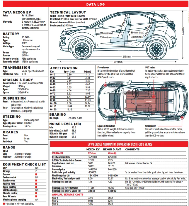
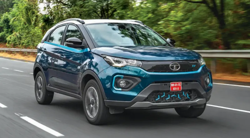
• The above mentioned TATA NEXON EV is modeled in Simulink: Specifications of TATA NEXON EV: ( claimed on test conditions)
• 
• 
• 
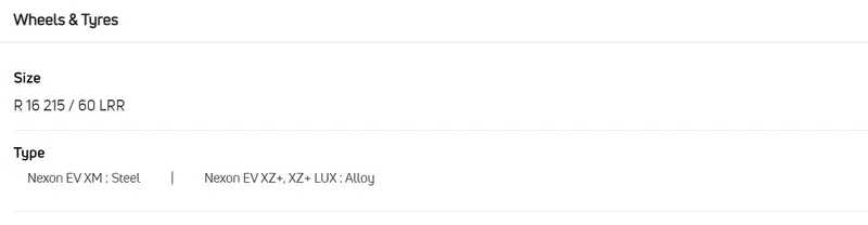
• More detailed specifications along with features:
• 
• 
• As per ARAI test data the vehicle has been tested for Modified Indian drive cycle (highways).
• a) Drive cycles
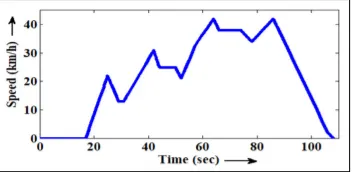
• A driving cycle is a series of data points representing the speed of a vehicle versus time. Driving cycles are produced by different countries and organizations to assess the performance of vehicles in various ways, as for instance fuel consumption, electric vehicle autonomy, and polluting emissions.
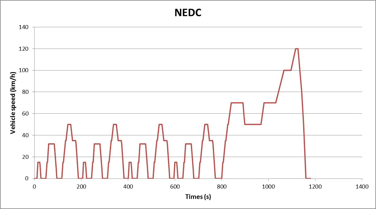
• Here the simulation is carried out for NEDC as well as IDC (Urban). The NEDC drive cycle has a top speed of 120 kmph but due to large idling time currently testing is carried out for WLTP Class 3 that is in line with EURO 7 standards. In India BS 6 is followed which has less top speed compared to WLTP Class 3. Though it is hard to realize this a simulation has been done on this as well. The main two drive cycles are NEDC and IDC (Urban)

• NEDC

  

• The NEDC is used as a reference cycle for homologating vehicles until Euro6 norm in Europe and some other countries. It is made of an urban part called ECE, which is repeated four times, and an extra-urban part, the EUDC. Here are the main characteristics of the cycle:

  Distance	11023 m
  Duration	1180 s
  Average speed	33.6 km/h

• IDC (Indian drive cycle)
• 
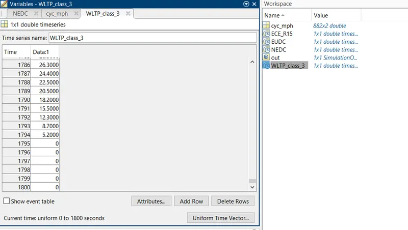
• The reference drive cycle data is loaded on matlab workspace:
• 
• b) Vehicle modeling and blocks uses
• 
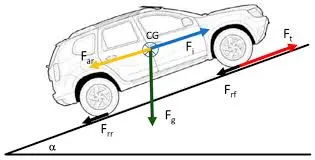
• Vehicle dynamic modelling-By using Newton’s law of motion, the vehicle is modeled as a load by considering various longitudinal forces acting on it.
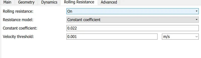
• The values for different parameters such as Kerb Weight (kg), Payload (kg), Coefficient of rolling resistance, Air density (kg/m3), Width (m), Height (m), Drag coefficient were taken from the spec sheet of cars namely:
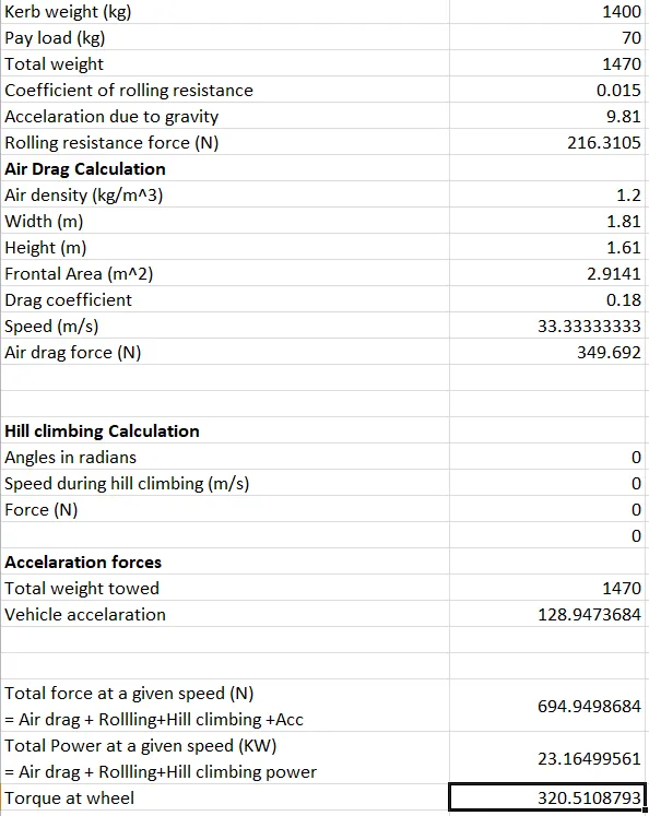
• Force due to rolling resistance,Frr= Urr*m*g where Urr is the Coefficient of rolling resistance,m is the sum of kerb weight and payload, g is the acceleration due to gravity
• Force due to aerodynamic drag, Fa= 1/2*p*A*V^2, p is Air density, A is Frontal area,V is the velocity of air stream flowing around the body
• Force due to hill climb, Fhc=m*g*sin(psi),m is sum of kerb weight and payload, g is the acceleration due to gravity,psi is the angle in radians
• The tractive force, Ft, required to drive the wheels by overcoming resistive force is given by Ft = Frr + Fad + Fhc +Fla +Fva, where Frr is the rolling resistance force, Fad is the aerodynamic drag, Fhc is the hill-climbing force, Fla is the
  linear acceleration force and Fva is the rotational acceleration force
• Using the obtained instantaneous tractive forces and the speed of the vehicle, the tractive power required at wheels is calculated as
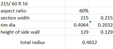
  Tractive power, Pt = Ft*v
• Wheel radius calculation: How to read a tire
• 
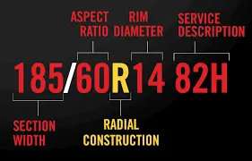
• Total wheel diameter= rim diameter + 2*height of sidewall
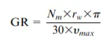
• Gear ratio=Nm*rw*pi/60*Vmax
• Wwheel=( V/r)*G
• The required wheel torque can be calculated from, T req = FT*rw.
• For Nexon EV considering all parameters the tractive effort has been determined for its top speed of 120 km/ hr( approximations have been done):
• Wheel dimensions:
• 
• Tractive effort at the top speed for the acceleration prescribed in NEDC:
• 
• The Gear ratio for above is 5.39 (evaluated based on ). The maximum motor speed data is not available hence assumption has been made. Though it is claimed that the top speed can be reached in 9.9 sec based on research from a web source it is found that 100 km/hr speed takes about 10 s.
• The gear ratio for peak torque according to specifications is about 6.39. The final drive ratio possible is 9.1:1
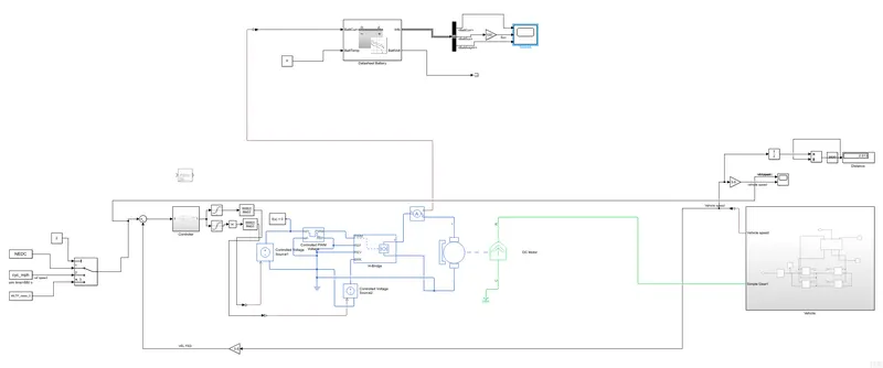
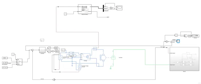
• The model made in Simulink to represent the vehicle subsystem as follows:
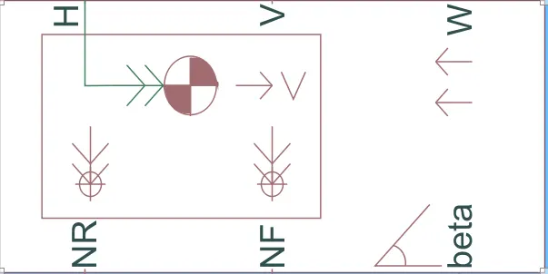
• The vehicle specifications and factors that contribute to resistive forces are input into the below block called vehicle body.
• 

• The block represents a two-axle vehicle body in longitudinal motion. The block accounts for body mass, aerodynamic drag, road incline, and weight distribution between axles due to acceleration and road profile. The vehicle can have the same or a different number of wheels on each axle. Connection H is the mechanical translational conserving port associated with the horizontal motion of the vehicle body. The resulting traction motion developed by tires should be connected to this port. Connections V, NF, and NR are physical signal output ports for vehicle velocity and front and rear normal wheel forces, respectively.

• vehicle body parameters:
• 
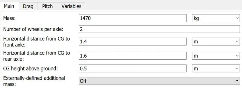
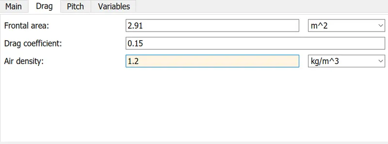
• Gear ratio=Nm*rw*pi/60*Vmax
• The gear system is obtained via a simple gear block.It represents a fixed-ratio gear or gearbox. No inertia or compliance is modeled in this block. You can optionally include gear meshing and viscous bearing losses. The gear ratio is varied for the reference velocity to match the output.
• 
• 
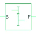
• A lower (taller) gear ratio provides a higher top speed, and a higher (shorter) gear ratio provides faster acceleration. Here a low drive ratio is used compared to max possible value as mentioned by the company where the acceleration time to claimed top speed is less.
• 
• Interia block- The block represents an ideal mechanical rotational inertia.
• 
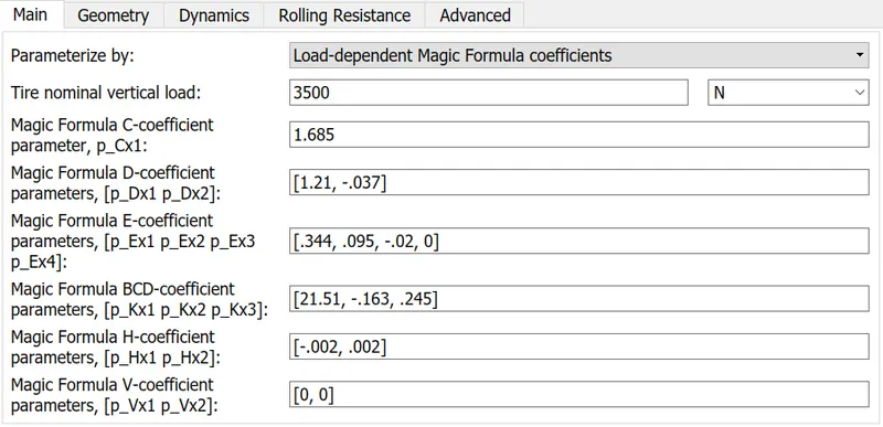
• The tires are represented by: Represents the longitudinal behavior of a highway tire characterized by the tire Magic Formula.
• 
• In tires the magic formula evaluates forces by peak longitudinal forces acting on the vehicle. The inside parameters are given as:
• The four-wheeler has a vertical load of W/4 acting on each tire
• The vehicle dynamics which can be also called as vehicle dynamics blocks that produce the velocity as a response to drive cycles are represented below. Here in-vehicle block zero gradients and wind speed are given 0 values via ps constant block.
• 
• Vehicle subsystem
• 
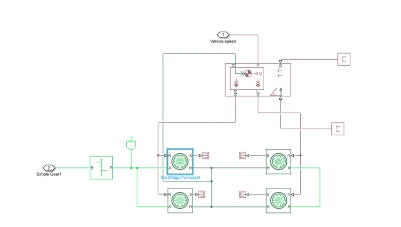
• The output of the subsystem is the vehicle velocity which is compared with the reference drive cycle to initiate acceleration and retardation commands to drive the motor which matches the speed according to driver inputs.
• c) Motor selection
• A permanent magnet DC motor is used as it is intended for LEVs. It exhibits better performance in terms of efficiency, fast response, simple structure, high torque, and easier maintenance.
• Then, the motor power is calculated from the tractive power using motor power, Pm = Pt/nt where nt is the efficiency of transmission. The transmission efficiency is assumed as 95%.
• Any motor can operate above its rated voltage value for some amount of time.
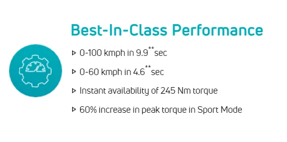
• The peak motor power is about 94 KW. The motor can produce:
• 
• Rated motor speed calculation:
• 
• 
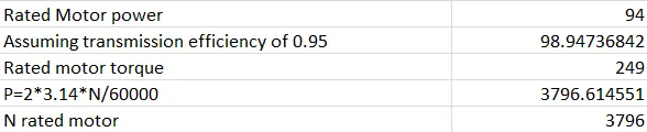
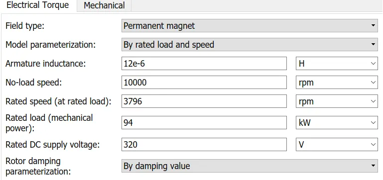
• The value of acceleration forces yields more power and must be given from the battery source. The top speed is according to the drive cycle is met by adjusting the motor controller and PWM source.
• d) Motor controller and PWM Block
• A power electronic converter is an electronic device made of high-power semiconductor switches that use different switching states to change the magnitude and waveform of voltage between input and output. Power converter circuits are used to control the flow of energy by supplying the right amount of current and voltage with help of power semiconductor switches. Power electronics deals with the conversion and control of electrical energy with the help of power semiconductor devices that operate in a switching mode, and, therefore, the efficiency of power electronic apparatus may approach as high as 98–99%. They can be uni or bidirectional.
  There are four possible types of power electronics converters namely
  a) AC to DC converters (controlled rectifiers).
  b) AC to AC converters (AC voltage controllers).
  c) DC to AC converters (Inverters).
  d) DC to DC converters (DC choppers).
• PE circuits can apply power varying from tens of watts up to hundreds of megawatts. They have high energy conversion efficiency. In a power electronic circuit, there exists only periodic linking of a power source to the load. This acts like an ideal switch where during an on the state there is null resistance and during off state, there is infinitesimally high resistance. The usage is preferred due to the absence of dissipation elements and power losses being nearly equal to zero. The duty cycle of a signal measures the fraction of time a given transmitter is transmitting that signal. This fraction of time determines the overall power delivered by the signal. Signals with longer duty cycles carry more power. This makes the signal stronger, more reliable, and easily detected by receiving equipment. Signals with longer duty cycles require less efficient receivers than do signals with shorter duty cycles.
• Depending upon maximum acceleration and retardation values in a duty cycle, the values must be chosen to step up and step down voltages.
• H-Bridge- This block represents an H-bridge motor drive. The block can be driven by the Controlled PWM Voltage block in PWM or Averaged mode. In PWM mode, the motor is powered if the PWM port voltage is above the Enable threshold voltage. In Averaged mode, the PWM port voltage divided by the PWM signal amplitude parameter defines the ratio of the on-time to the PWM period. Using this ratio and assumptions about the load, the block applies an average voltage to the load that achieves the correct average load current. The Simulation mode parameter value must be the same for the Controlled PWM Voltage and H-Bridge blocks.
• During regenerative braking, the battery is charged. During the deceleration stage, energy should be recovered from the machine. For this purpose, the power converter must be bidirectional in current in order to ensure regenerative braking during deceleration stages. The motor drive's operation is performed.
• H-Bridge parameters -
• 
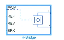
• The voltage to the H bride,gate pulses must be controlled according to reference input for that a controlled PWM block us used and its user defined parameters are described below. The power setting is set as internal
• 
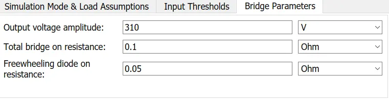
• Controlled PWM Block-This block creates a Pulse-Width Modulated (PWM) voltage across the PWM and REF ports.
• 
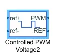
• PWM Block parameters- switching frequency represents how many times the pulses are given to open and close the h bridge
• 
• 
• 
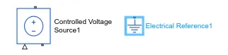
• In simscape the negative terminals are grounded via an electrical reference and to main a constant voltage across a physical connected a control voltage source block is used.
• 
• The motor along with the control and pwm source is represented as below:
• 
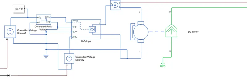
• The input to the controlled voltage source is the acceleration and deceleration command from the longitudinal controller which is a PID controller.
• e) PID Control
• The basic idea behind a PID controller is to read a sensor, then compute the desired actuator output by calculating proportional, integral, and derivative responses and summing those three components to compute the output PID control is used to establish reference tracking. A drive cycle represents the instance velocity of the vehicle at various instant of time. The aim of using a controller is to establish control over the output velocity such that the input reference velocity is tracked.
• PID theory

• Proportional Response
  The proportional component depends only on the difference between the setpoint and the process variable. This difference is referred to as the Error term. The proportional gain (K_p) determines the ratio of output response to the error signal. For instance, if the error term has a magnitude of 10, a proportional gain of 5 would produce a proportional response of 50. In general, increasing the proportional gain will increase the speed of the control system response. However, if the proportional gain is too large, the process variable will begin to oscillate. If K_c is increased further, the oscillations will become larger and the system will become unstable and may even oscillate out of control.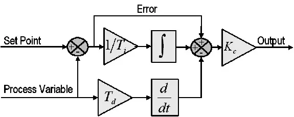

  
  Block diagram of a basic PID control algorithm.

  
  
  Integral Response (K_i)
  The integral component sums the error term over time. The result is that even a small error term will cause the integral component to increase slowly. The integral response will continually increase over time unless the error is zero, so the effect is to drive the Steady-State error to zero. Steady-State error is the final difference between the process variable and setpoint. A phenomenon called integral windup results when integral action saturates a controller without the controller driving the error signal toward zero.
  
  Derivative Response (K_d)
  The derivative component causes the output to decrease if the process variable is increasing rapidly. The derivative response is proportional to the rate of change of the process variable. Increasing the derivative time (T_d) parameter will cause the control system to react more strongly to changes in the error term and will increase the speed of the overall control system response. Most practical control systems use very small derivative time (T_d), because the Derivative Response is highly sensitive to noise in the process variable signal. If the sensor feedback signal is noisy or if the control loop rate is too slow, the derivative response can make the control system unstable

• How to tune a PID:
• 
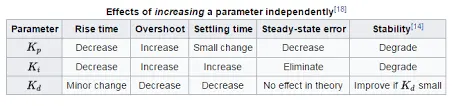
• Intially the PID was autotuned to get particular set of Kp,Ki and Kd values then it was fine-tuned by manually inputting values. Following this the control system as represented above in the schematic was made in simulink as shown below.
• 
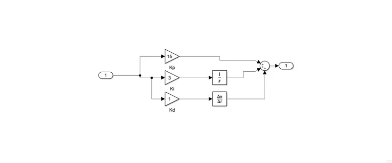
• The PI values are adjusted for output to track the reference input.
• f) Battery system
• The battery pack with the terminal voltage of 320 V is directly connected to the motor drive. The current is sensed from the motor in real-time and a system is created to measure the SOC when a drive cycle is used. The battery capacity is estimated as a product of battery voltage and battery capacity which is 94 Ah. This is rated capacity but battery capacity will be a bit more.
• To represent a battery system a DC battery block is used, which is grounded and it receives motor current requirement as an input which is sensed through a current sensor.
• Battery capacity estimation:
• 
• It is assumed that the nominal voltage of a cell used to make the battery pack is 3.7 V. Considering all losses that will incur a battery pack voltage of 347 is assumed above the rated value as in performance mode the vehicle can be operated 60% peak value
• The following calculations are going to be performed for each cell type. For this example, we are going to consider that the battery pack is made up only of several strings connected in parallel.
• Number of cells connected in series= Battery pack voltage / Voltage of single cell= 320/3.7= 94.07 approximated to 86
• Energy content represented by each series combination = number of cells connected in series* energy of each cell
• One cell has a capacity of 1.1 Ah. Hence the number of parallel string for required energy is 1
• The combination used is 86 S and 1 P
• The battery is represented by a datasheet battery model:
• 
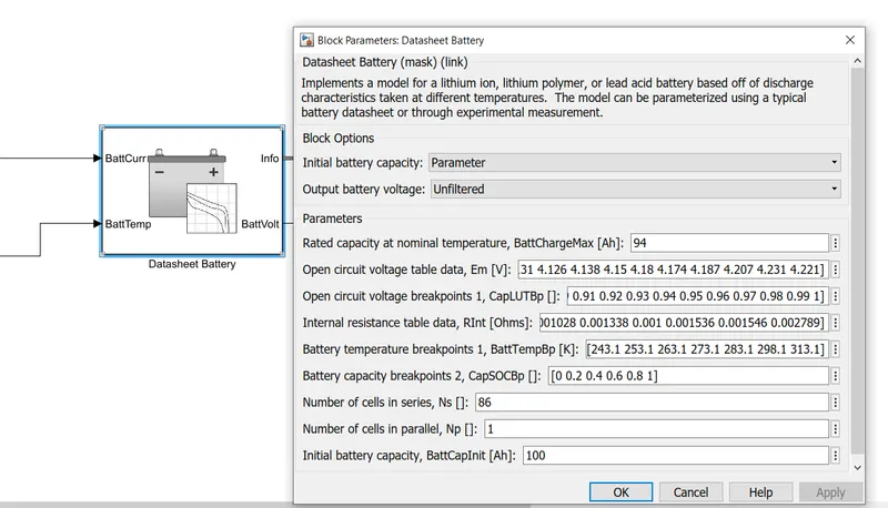
• The battery current is input from the current sensed from the motor and the constant 0 blocks is given to battery temperature. Using a bus selector block the values of the battery such as soc, capacity, and current drawn are sensed.
• Apart from the rated capacity values and battery construction that has been calculated all other values are taken which were in the block as default
• There is a need to estimate the State of Charge at the end of drive cycles for which the system is tested.
• Hence a measurement system is made.
• The drive cycle is input with help of a multiport switch which can be chosen. Say there are 3 drive cycle to be checked
• All three are input to multiport switch.
• There is an import where a constant block can be attached
• If the second drive cycle in the sequence has to be simulated then the corresponding number is kept in the constant block.
• Three standard drive cycles used
• To run a drive cycle simulation from Matlab workspace using a from workspace block is used
• A solver configuration block is also used in the system
• 
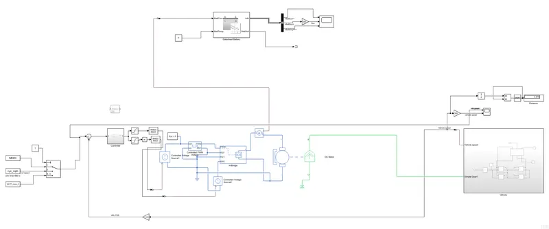
• 4) Results and Inference (Simulink Model for Tata Nexon ziptron)
• 1) NEDC CYCLE - The simulation time for the NEDC drive cycle is 1180 s
• a) Output window:
• 
• b) SoC, Current, and Capacity of Battery
• 
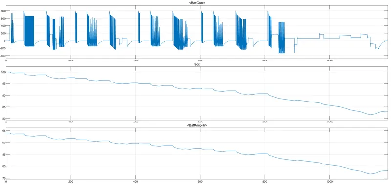
• c ) Reference speed and output vehicle speed
• 
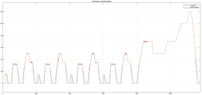
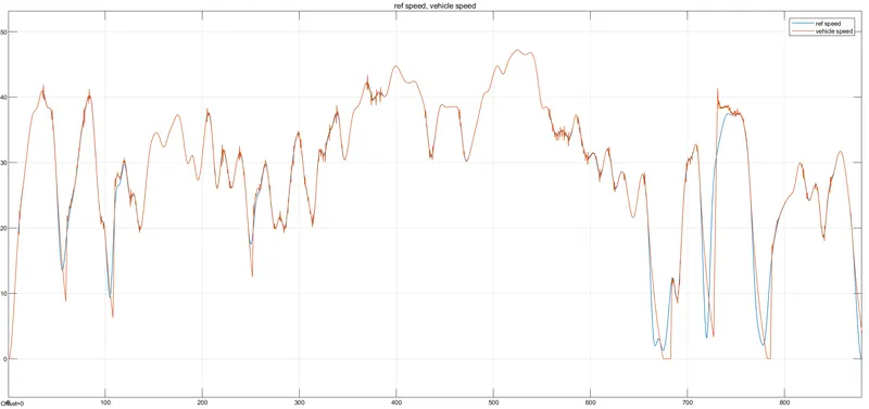
• 2) Indian drive cycle (Urban)-The simulation time for NEDC drive cycle is 880 s
• a) Output window:
• 
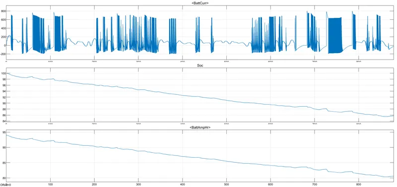
• b) SoC, Current, and Capacity of Battery
• 
• c) Reference speed and output vehicle speed
• 
• 3) WLTP drive cycle-The simulation time for NEDC drive cycle is 1800 s
• a) Output window:
• 
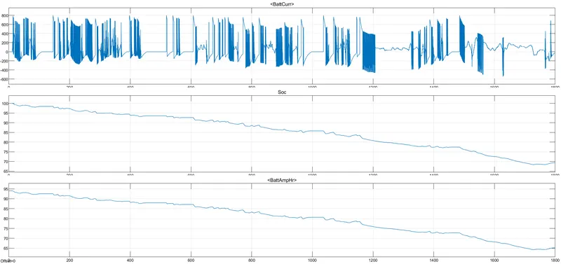
• b) SoC, Current, and Capacity of Battery
• 
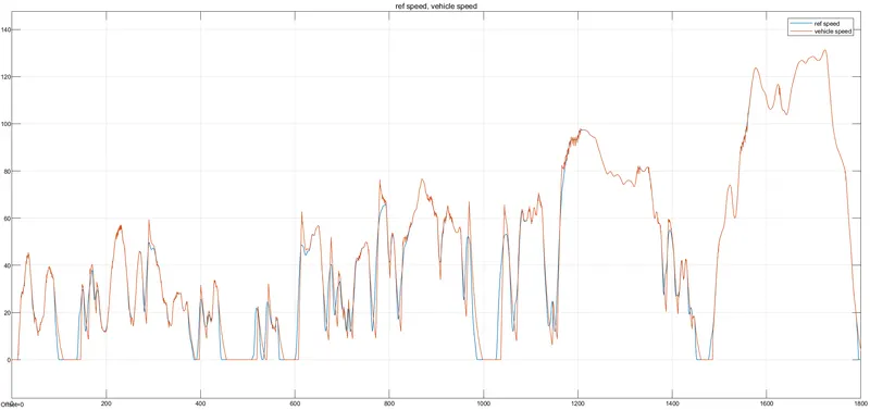
• c) Reference speed and output vehicle speed
• 
• 5) Conclusions ( from above graphs)

• Drive cycle	SOC %	Energy consumed during drive cycle	Distance covered (Km)	Inference
  NEDC (1180)	82.5	17 Ah approx	3.078	The top speed is reached. Till the first 800 s the drive cycle has many identical speed patterns of acceleration. There is a lag to reach the lower speed values this might be due to the Kp,Ki, and Kd values selected. The values set for Kp is high as it was needed to meet the top speed in the cycle. The instance of a top speed of a vehicle of 120kmph is at end of the drive cycle. From the current pattern, there are indications of regeneration. The response to lower speeds is less.The overshoot at low speeds is an indication that the kd values chosen must be increased and the Ki value must be decreased.
  WLTP Class 3 (1800)	69	29 Ah approx	6.48	The required drive cycle is matched. From the specs, it was evident that it is possible to operate the vehicle above top speed but the back emf effect will be there. These are shot times when the motor can offer the power of up to 60% of its peak rated power. This affects the SOC of the battery. From 1500 to 1800 s the vehicle is continuously operated at a power that is more than the peak. This has affected the SOC. This can be understood from the SOC graph where there is a steep decline. Sometimes at instances of top speed and low speed, the vehicle speed is exceeding reference values which a case of overshoot and is due to the high value of Kp
  Urban Indian (881s)	85.55	12 Ah approx	2.013	The Indian drive cycle has many retardations and start-stop operations. There are instances where the vehicle is accelerated after a decrease in speed. The drive-in urban features idling which takes energy from the battery a lot. number But the distance covered compared to the other two is less.. This is mostly a start-stop operation in a city and the vehicle is driven at low speed.

• To tune a PID use the following steps:

  1. Set all gains to zero.
  2. Increase the P gain until the response to a disturbance is steady oscillation.
  3. Increase the D gain until the oscillations go away
  4. Repeat steps 2 and 3 until increasing the D gain does not stop the oscillations.
  5. Set P and D to the last stable values.
  6. Increase the I gain until it brings you to the setpoint with the number of oscillations desired
• 6) Learning outcome
• - It is possible to operate a vehicle beyond a mentioned peak speed
• - Drive ratios are dependant on the drive cycles
• - SoC though is dependant on driving patterns. If in a drive cycle at multiple times the vehicle is operated at an intermittent zone of motor operation the SoC falls drastically
• - It is not advisable to use Kp, Ki, and Kd values as same for each drive cycle. The proportional rise and Ki which is an indication of the history of error is dependant on the reference signal which varies in each drive cycle.
• - Motor sizing and calculation
• 7) References
• - https://nexonev.tatamotors.com/features/
• -https://www.tatamotors.com/wp-content/uploads/2021/01/07060255/media-01jan21.pdf
• -Modelling, design and control of a light electric vehicle with hybrid energy storage system for Indian driving cycle
• -Efficient Gear Ratio Selection of a Single-SpeedDrivetrain for Improved Electric Vehicle Energy Consumption
• -https://www.rhydolabz.com/hardwares-batteries-c-170_167/polymer-lithium-ion-battery-1000mah-p-556.html
• -https://www.sparkfun.com/datasheets/Batteries/UnionBattery-1000mAh.pdf
• - - https://x-engineer.org/automotive-engineering/vehicle/electric-vehicles/ev-design-battery-calculation/

Google drive links-

1) Simulink model- https://drive.google.com/file/d/1Q8iBdkoRh3r_3lxevpRfOE-NaRhagjuy/view?usp=sharing

2) .m file for drive cycles- https://drive.google.com/file/d/1Q8iBdkoRh3r_3lxevpRfOE-NaRhagjuy/view?usp=sharing

3) Motor sizing calculations - https://drive.google.com/file/d/1LgIVoWtaAxLsZGxKb_XI1G99oadrw76q/view?usp=sharing