Week 4 - Genetic Algorithm
AIM
To write a code in MATLAB to optimise the stalagmite function and find the global maxima of the function
Theory
- Basic defition
A genetic algorithm has been derived on the basis of Charles Darwin’s theory of natural evolution. The alogorithm is synonymous to natural selection where in fittest individuals are choses for procreatopm of new offspring and there by next generation. For a given population natural selection work selection of fittest individuals from a population. The selected ones produce offspring which inherit the characteristics of the parents and will be added to the next generation.Depending on the fitness of parents the offsprings have a better survival rate and the process is iterated till a generation with fittest individuals are found.
2. How it works
Five phases are considered in a genetic algorithm.
a) Initial population- The process starts with a set of individuals called as population.An individual is characterized by a set of parameters (variables)
b) Fitness function-The fitness function determines how fit an individual is. The fitness value of an individual is the value of fitness function
From selection process to mutation the evaluation is explained with example to parents p1 and p2
c) Selection- Retaining the best performing individuals.Two pairs of individuals (parents) are selected based on their fitness scores. Individuals with high fitness have more chance to be selected for reproduction.The best are taken for cross over
d) Crossover-For each pair to be mated a randomn cross over point os chosen. For example :
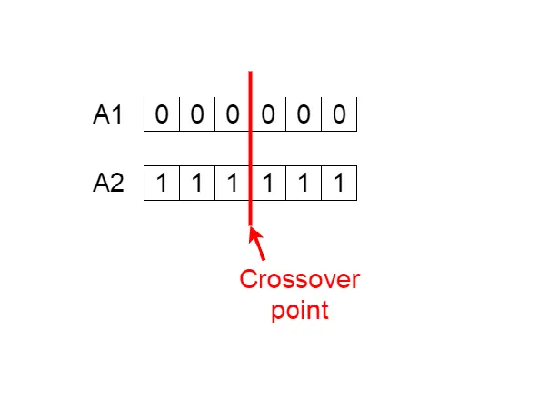
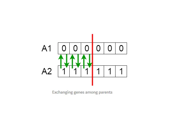
offspring are generated by exchanging genes among parents.
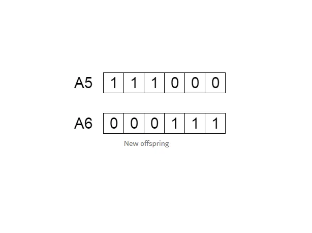
The new off springs are produced
e) Mutation-Mutation is done to maintain diversity with the population and to prevent the occurance of a convergence prematurely
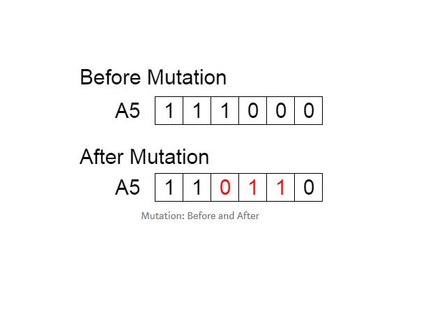
The alogrithm terminates once the convergence is obtained.
c) Mathematical definition and operation of GA-Genetic Algorithm (GA) is an optimization technique based on the principles of Genetics and Natural Selection. It is frequently used to find optimal or near-optimal solutions It is used to solve optimization problems, in research, and in machine learning.Optimization is the process of finding the values of inputs in such a way that the “best” output values. The definition of “best” is dependant on a problem. Mathematically it refers to maximizing or minimizing one or more objective functions, by varying the input parameters.
The set of all possible solutions or values which the inputs can take make up the search space. In this search space, lies a point or a set of points which gives the optimal solution. The aim of optimization is to find that point or set of points in the search space. Due to its randomn narure the algorithm provides a local minima than a global minima.
Optimization is the process of finding the point that minimizes a function. There exists a Global minima as well as a local minima. Global minima refers to entire domain where as local minima is at the immediate neighbourhood.The genetic algorithm can the deficiency with the right settings.
3. Explaination of syntax for GA:
a) x = ga(fun,nvars,A,b,Aeq,beq,lb,ub)
fun - Function-user defined
nvars- number of variables
A-Linear inequality constrains
b-Linear inequality constrains
Aeq-Linear equality constrains
Beq-Linear equality constrains
lb-Lower bounds of the variables
up-Upper bounds of the variables
b) x = ga(fun,nvars,A,b,[],[],lb,ub,nonlcon,IntCon,options)
fun - Function-user defined
nvars- number of variables
A-Linear inequality constrains
b-Linear inequality constrains
Aeq-Linear equality constrains
Beq-Linear equality constrains
lb-Lower bounds of the variables
up-Upper bounds of the variables
nonlcon-Non linear constrains
IntCon-Integer variables
Options-Optimization options
4)Code ,Explaination and Output The function that has to be
optimized is :
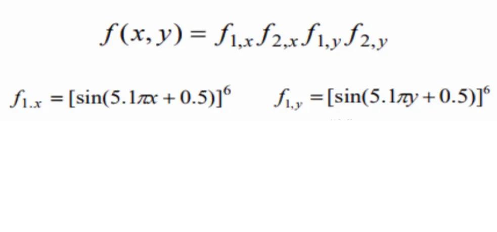
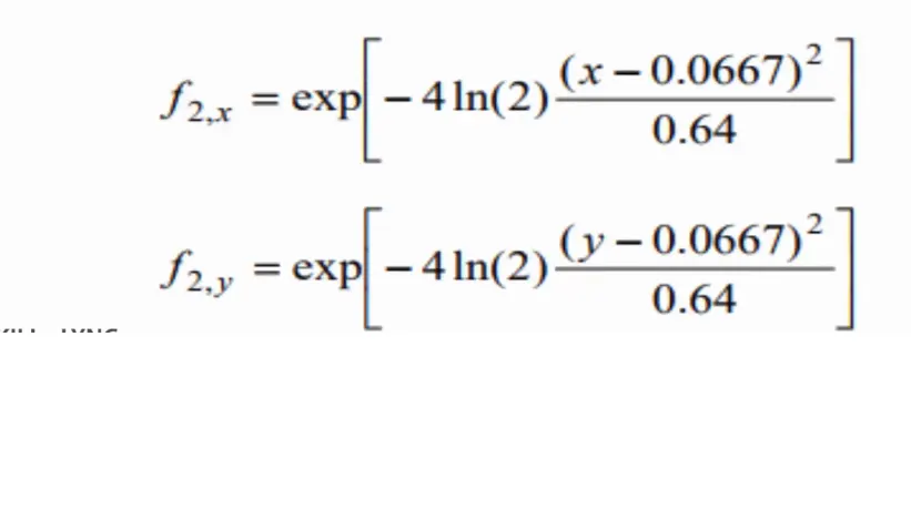
To form the stalagmite function intially a user defined function is created:
function [f] = stalagamite(input_vector)
 x=input_vector(1);
 y=input_vector(2);
 f1_x=(sin(5.1*pi*x+0.5))^6;
 f1_y=(sin(5.1*pi*y+0.5))^6;


 f2_x=exp(-4*log(2)*((x-0.0667)^2)/0.64);


 f2_y=exp(-4*log(2)*((y-0.0667)^2)/0.64);

 f_0=(f1_x*f2_x*f1_y*f2_y);
%   f=1/(1+f_0);
 f=-f_0;
end
The genetic algorithm yields the local minima and global minina of a function but the requirement is to find the Global maxima. Hence the fuction defined as 'F IS REDEFINED AS -F_0 AS IT GIVES GLOBAL MAXIMA'
Final code:
clear all
close all
clc
no_cases=50;
x=linspace(0,0.6,150);
y=linspace(0,0.6,150);
%number of iterations are specified so that ga knows the search space
% creation of multidimensional array
[xx, yy]= meshgrid(x, y);


% plot for stalagamite function
 for i=1:length(xx)
     for j=1:length(yy)
         input_vector(1)=xx(i,j);
         input_vector(2)=yy(i,j);
         f(i,j)= stalagamite(input_vector);
     end
 end
 surfc(xx,yy,f)
 shading interp
 [inputs,fvar]=ga(@stalagamite, 2);
% study of statistical behaviour for 50 iterations

% study 1
tic
for i=1:no_cases
    [inputs,fopt(i)]=ga(@stalagamite,2);
    % optimum x and y values are stored
    xopt(i)=inputs(1);
    yopt(i)=inputs(2);
end
study1_time=toc;
figure(1)
subplot(2,1,1)
hold on
surfc(x,y,f)
shading interp
plot3(xopt,yopt,-fopt,'marker','o','markersize',5,'markerfacecolor','r')
title('Unbounded inputs')
subplot(2,1,2)
plot(-fopt)
xlabel('Iterations')
ylabel('Function maximum')
% study 2 the variables  are set upper and lower bounds to avoid
% fluctuating minima values
% syntax for ga- x = ga(fun,nvars,A,b,Aeq,beq,lb,ub)
tic
for i=1:no_cases
    [inputs,fopt(i)]=ga(@stalagamite,2,[],[],[],[],[0;0],[0.6;0.6]);
    % optimum x and y values are stored
    xopt(i)=inputs(1);
     yopt(i)=inputs(2);
end
study2_time=toc;
figure(2)
subplot(2,1,1)
hold on
surfc(x,y,f)
shading interp
plot3(xopt,yopt,fopt,'marker','o','markersize',5,'markerfacecolor','r')
title('Unbounded inputs')
subplot(2,1,2)
plot(fopt)
xlabel('Iterations')
ylabel('Function maximum')

% study 3-Incresing population size(iterations as well) to determine global minima
% new syntax -x = ga(fun,nvars,A,b,[],[],lb,ub,nonlcon,IntCon,options)
options= optimoptions('ga');
options= optimoptions(options,'PopulationSize',1000);

tic

for i=1:no_cases
    [inputs,fopt(i)]=ga(@stalagamite,2,[],[],[],[],[0;0],[0.6;0.6],[],[],options);
    % optimum x and y values are stored
    xopt(i)=inputs(1);
    yopt(i)=inputs(2);
end
study3_time=toc;
figure(3)
subplot(2,1,1)
hold on
surfc(x,y,f)
shading interp
plot3(xopt,yopt,-fopt,'marker','o','markersize',10,'markerfacecolor','r')
title('Unbounded inputs')
subplot(2,1,2)
plot(-fopt)
xlabel('Iterations')
ylabel('Function maximum')
a) The sample space for variables x and y are defined as (0,0.6,150)
b) A multidimensional array of [xx,yy] is created with meshgrid command
c) As the ga command used does not identify iteration it must do in the search space a variable called as no_cases is defined and the value is set as 50
d) to obtain a Global maxima value 3 statistical studies are carried out
e) Statistical study 1- Initially to study the statistical behaviour a for loop is inititated which does 50 iterations for different values of x and y. Before starting loop tic command is used to start stop watch timer
1)within for loop which has i that scans through each iteration, [input,fopt(i)]=ga (@stalagamite,2) is used in each ith case of iteration fopt value is found. For each 'i' xopt and y opt values are found which is equal to inputs 1 and inputs 2 that are previously defined.This is used to calculate fopt value
2) A subplot is made on figure 1 which divides the plane into four quadrants. In subplot(2,1,1) a surface plot is made with shading interp which shows lines on surface(x,y,-fopt). Apart from this a 3D plot is made with plot3 command between xopt,yopt and -fopt.
3) In the second position of subplot (2,1,2) plot of -fopt is made with y axes as maximum value of function and x as the 50 iterations so that it helps to show whether maxima is a single point or is it fluctuating creating an error
4) toc command is used to stop the timer and the run time for iteration is stored in study1_time
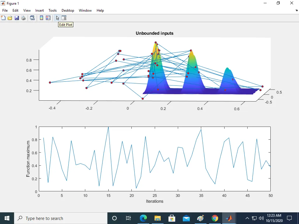
output study 1: In study 1 it was found that during each iteration the value was fluctuating.
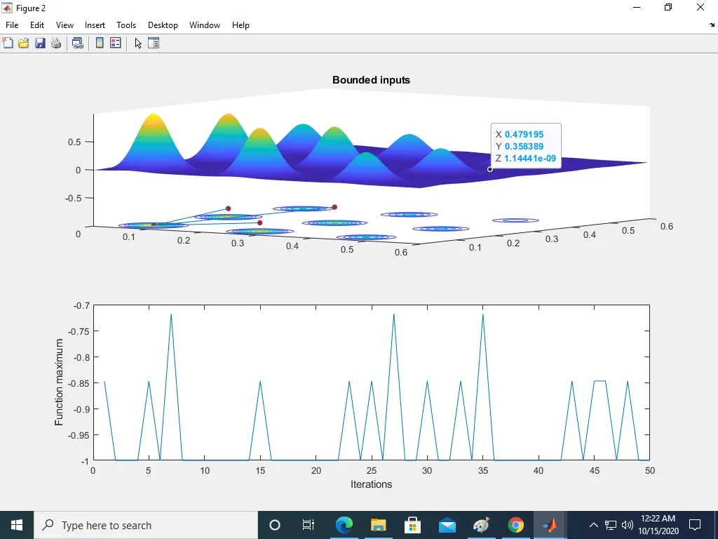
f) Statistical study 2 : Since the Maxima value was found to be fluctuating, upper and lower bounds are set for the defined variables x and y
1) The syntax used is defined in theory part.
syntax for ga- x = ga(fun,nvars,A,b,Aeq,beq,lb,ub) lb for x,y: 0,0 upper bound for x,y=0.6,0.6
2) Within for loop which has i that scans through each iteration, [inputs,fopt(i)]=ga(@stalagamite,2,[],[],[],[],[0;0],[0.6;0.6]) is used in each ith case of iteration fopt value is found. For each 'i' xopt and y opt values are found which is equal to inputs 1 and inputs 2 that are previously defined. This is used to calculate fopt value
3) A subplot is made on figure 2 which divides the plane into four quadrants. In subplot(2,1,1) a surface plot is made with shading interp which shows lines on surface(x,y,-fopt). Apart from this a 3D plot is made with plot3 command between xopt,yopt and -fopt.
4) In the second position of subplot (2,1,2) plot of -fopt is made with y axes as maximum value of function and x as the 50 iterations so that it helps to show whether maxima is a single point or is it fluctuating creating an error
5) toc command is used to stop the timer and the run time for iteration is stored in study2_time
Output study 2: For an optimization problem, when maximized it can have only one global maxima and not many in number. In study 2 4 maximums were observed on 3D plot . The fopt had four peaks in 3D plot.
g) Statistical study 3 :There is a need to mention a population size.
1) The syntax used is defined in theory part.
Prior to starting for loopwhich calculates the value for -fopt for each ith case of x and y a population size is defined. The code for the same is:
options= optimoptions('ga'); this refers to options available to optimze ga
options= optimoptions(options,'PopulationSize',1000);
x = ga(fun,nvars,A,b,[],[],lb,ub,nonlcon,IntCon,options) lb for x,y: 0,0 upper bound for x,y=0.6,0.6. Options refers to optimization option
2) Within for loop which has i that scans through each iteration, [inputs,fopt(i)]=ga(@stalagamite,2,[],[],[],[],[0;0],[0.6;0.6],[],[],options)is used in each ith case of iteration fopt value is found. For each 'i' xopt and y opt values are found which is equal to inputs 1 and inputs 2 that are previously defined. This is used to calculate fopt value
3) A subplot is made on figure 2 which divides the plane into four quadrants. In subplot(2,1,1) a surface plot is made with shading interp which shows lines on surface(x,y,-fopt). Apart from this a 3D plot is made with plot3 command between xopt,yopt and -fopt.
4) In the second position of subplot (2,1,2) plot of -fopt is made with y axes as maximum value of function and x as the 50 iterations so that it helps to show whether maxima is a single point or is it fluctuating creating an error
5) toc command is used to stop the timer and the run time for iteration is stored in study2_time
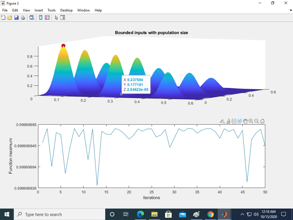
Output study 2: With an increased population size of 1000, it was possible to obtain a global maxima for the function
5) Result:
The maximum value of function was found to be 0.999999835. There was only one peak observed the 3D plot and the fluctuation of Fopt max value for iteration was minmal. A wel defined population size combined with options syntax for optimization yields better results.
6) Screen shot of output
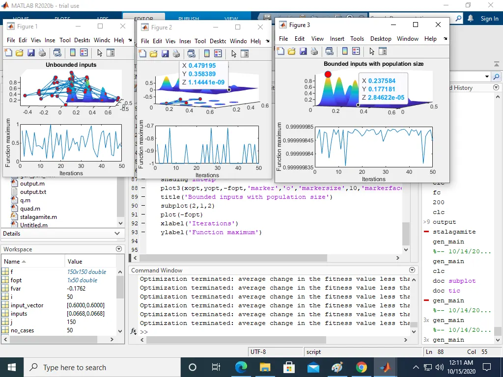
GA_Study_3 with population size of 1000
GA_Study_2 with lb and ub
GA_Study_1 for 50 iterations