Exploratory Data Analysis on Iris data set

Decision tree:

A decision tree is a supervised machine learning algorithm that can be used for both classification and regression problems. A decision tree is simply a series of sequential decisions made to reach a specific result.

A decision tree has root nodes, children nodes, and leaf nodes, where each node attribute is decided based on its information gain or Gini impurity.

Random forest:

A decision tree is the building block of a random forest and is an intuitive model. Since decision trees are prone to overfitting, other tree-based models like Random Forest and XGBoost are preferred.

When training, each tree in a random forest learns from a random sample of the data points. The samples are drawn with replacement, known as bootstrapping, which means that some samples will be used multiple times in a single tree.

In a random forest algorithm, the following takes place:

1. Random sampling of training data points when building trees
2. Random subsets of features considered when splitting nodes

2.

Advantages

1. Powerful and highly accurate
2. No need for normalizing
3. Can handle several features at once
4. Run trees in parallel ways

Disadvantages

1. They are biased to certain features sometimes
2. Slow
3. Can not be used for linear methods

3. Classification is a supervised learning approach in which a target variable is discrete (or categorical).

Confusion matrix:

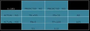
The above image depicts a confusion matrix, i.e. a table representing the actual values and the model predicted values.

The YES actual values for which the model has predicted YES is called True Positive and the NO actual values for which the model has predicted NO is called the True Negative.

The NO actual values for which the model has predicted YES is called the False Negative and is also referred to as Type-1 error whereas, the YES actual values for which the model has predicted NO is called the True Negative and is referred to as Type-2 error.

Accuracy: The accuracy of the model is determined based on its confusion matrix.

Accuracy = (TP+TN)/Total values

Precision: The precision of the model is the ratio of True Positive to the total YES predicted.

Precision = TP/Total YES = TP/(TP+FP)

True Positive Rate/Recall/Sensitivity: It is the ratio of True Positive outcomes to the number of actual YES outcomes.

True Positive Rate = TP/(TP+FN)

F1 score: F1 score is the weighted average of precision and recall.

F1 score is a more useful measure than accuracy for problems with uneven class distribution because it takes into account both false positives and false negatives.

The best value for the F1 score is 1 and the worst is 0.

ROC and AUC: ROC (receiver operating characteristics) curve and AUC (area under the curve) measures are used to evaluate a classification model’s performance.

ROC curve summarizes the performance of the model at different threshold values by combining confusion matrices at all threshold values. The x-axis of the ROC curve is the false positive rate (1- specificity) and the y-axis of the ROC curve is the true positive rate (sensitivity).

Specificity = TN/(TN+FP)

False positive rate = 1-TN/(TN+FP) = FP/(TN+FP)

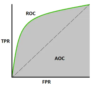
An excellent model has AUC near to the 1 which means it has a good measure of separability. A poor model has AUC near 0 which means it has the worst measure of separability.

4. Exploratory data analysis on Iris dataset

In statistics, exploratory data analysis is an approach to analyzing data sets to summarize their main characteristics, often using statistical graphics and other data visualization methods.

It refers to the critical process of performing initial investigations on data so as to discover patterns, to spot anomalies, test hypotheses, and to check assumptions with the help of summary statistics and graphical representations.

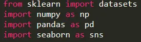
All the modules necessary for explorative, descriptive, predictive, and inferential analysis are imported.

Pandas: pandas is a fast, powerful, flexible, and easy-to-use open-source data analysis and manipulation tool, built on top of the Python programming language.

Seaborn: Seaborn is a Python data visualization library based on matplotlib. It provides a high-level interface for drawing attractive and informative statistical graphics.

Numpy: NumPy module works with numerical data and offers a powerful object called Array.

Loading the dataset:

Iris data set is loaded using datasets.load_iris() and assigned to the variable iris.

Printing the dataset:

By printing iris, we can see the data, target values, and the target names.

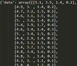
Target, which is an array consisting of 0,1 and 2, each corresponding to a particular class, which in this case is a type of Iris flower.

0 for Iris Setosa, 1 for Iris Versicolor, and 2 for Iris Virginica.

The data parameters are extracted using iris.data and assigned to a variable x. Similarly, all the target(output) values are assigned to y.

pd.DataFrame is used to view the data, and columns=['Petal length','Petal Width','Sepal Length','Sepal Width'] is used to assign a heading to each column.

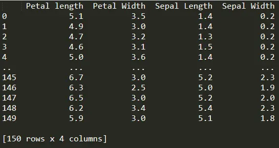
The dataset consists of 150 instances and 4 parameters(attributes).

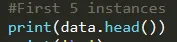
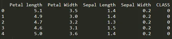
data.head() is used to view the first five instances. data.tail() is used to view the last five instances in the dataset.

data.describe is used to view the count, mean, standard deviation, minimum value, maximum value, 25th, 50th, and 75th percentile values of each feature in the dataset.

Descriptive statistics include those that summarize the central tendency, dispersion, and shape of a dataset’s distribution, excluding NaN values.

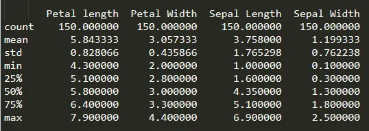
The mean petal length is 5.84 cm and has a max and min value of 7.9 and 4.3.

The mean petal width is 3.05 cm and has a max and min value of 4.4 and 2.0.

The mean sepal length is 1.76 cm and has a max and min value of 6.9 and 1.0.

The mean sepal width is 1.19 cm and has a max and min value of 2.5 and 0.1.

The info() function is used to print a concise summary of a DataFrame. This method prints information about a DataFrame including the index dtype and column types(Data types), non-null values, and memory usage.

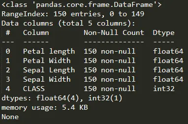
Data has only float and integer values.

No variable column has null/missing values.

isnull().valuesany() checks for any missing values in the parameters. It returned false, which meant that no data is missing.

isnull().sum() returns the number of missing values in the data set.

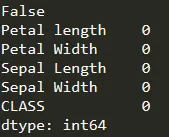
No missing values are present in the dataset.

Visualizing the dataset:

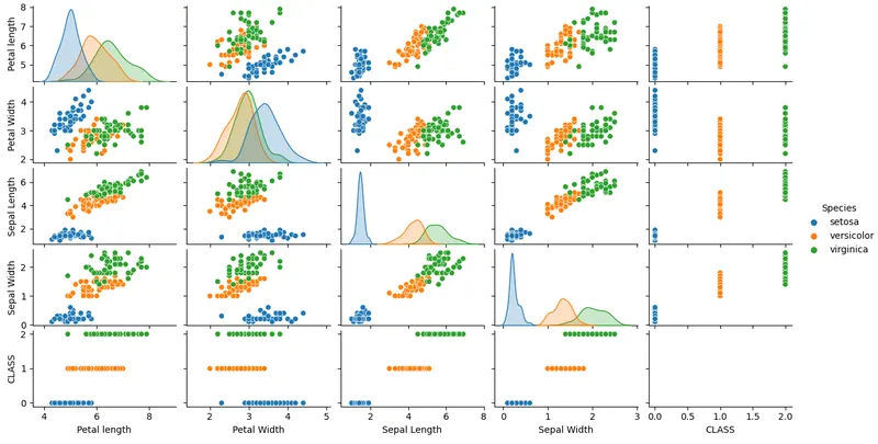
From the above plot, we can view the scatter plot of each attribute vs the remaining ones, and we can also view the standard deviation for all the attributes corresponding to each type of flower.

Degree of correlation:

To check how correlated each parameter is to one another.

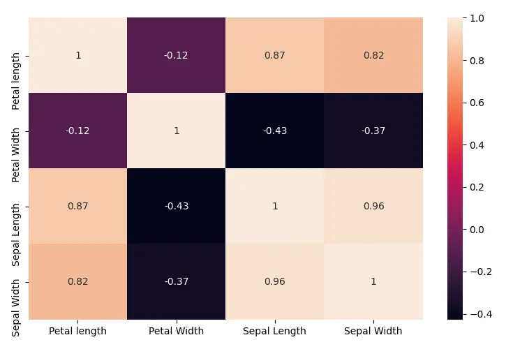
From the above plot, we can see that sepal length and sepal width have a high degree of correlation, i.e. of 0.96.

Highly correlated terms may be required to be eliminated in certain machine learning algorithms to avoid skewed or erroneous results.

References:

https://towardsdatascience.com/an-implementation-and-explanation-of-the-random-forest-in-python-77bf308a9b76

https://towardsdatascience.com/understanding-auc-roc-curve-68b2303cc9c5