Solving second order ODEs using Python

Aim: The aim of this challenge is to solve second order ODEs using Python.

Objectives: The objectives of this challenge is to

• Identifying the governing ordinary differential equations for a pendulum
• Solving the ODEs using Python
• Plotting the displacement and velocity profiles
• Simulate the damping effect on the pendulum by creating an animation

Theory:

Ordinary differential equation: It is an equation consisting of one or more derivatives of an independent variable. These equations have to solve to check what function or functions satisfy the equation.

In order to solve the ordinary differential equation, the equations have to be integrated. However, as the complexity of the differential equation increases, different methods have to be applied in order to solve the ODE, hence adding to the computational cost of solving it.

Order: It is the order of the highest derivative present.

Degree: The degree of a differential equation is the power of the highest derivative in the equation.

Ex:

1. `((overset(2)(d)y)/(overset(" "2)(dx))) = 2x`

Order = 2, Degree = 1

2. `overset(" "2)(((overset(2)(d)y)/(overset(" "2)(dx))) )+ overset(" "3)(((dy)/dx)) = 2x`

Order = 2, Degree = 2

ODE representing the motion of pendulum:

`((overset(2)(d)theta)/(overset(" "2)(dt))) + b/m*(d theta)/(dt) + g/L*sintheta = 0`

In the above equation,

g = gravity in m/s2,

L = length of the pendulum in m,

m = mass of the ball in kg,

b=damping coefficient.

Since the ODE is of order 2, it is broken down into two equations of the first-order ODE.

Let displacement `theta = theta1`

`(d theta)/dt = (d underset(1)(theta))/dt = underset(2)(theta)`

`(d underset(2)(theta))/dt = -(b/m)underset(2)(theta) - (g/l)sinunderset(1)(theta)`

Hence we have successfully broken down a 2nd order ODE into two first order ODE equations.

We will now solve these equations using odeint in python.

odeint uses inbuilt functions to integrate and solve for the values that satisfy the function.

Given Values:

L=1 metre,

m=1 kg,

b=0.05.

g=9.81 m/s2.

Initial Conditions:

At time t=0

Displacement = 0 rad

Angular velocity = 3 rad/s

Python Code:

#Python code to solver pendulum ODE
import math
from scipy.integrate import odeint
import numpy as np
import matplotlib.pyplot as plt


#Defining function
def model(theta,t,b,g,l,m):

	theta1 = theta[0]
	theta2 = theta[1]

	dtheta_1 = theta2
	dtheta_2 = -(b/m)*theta2-(g/l)*math.sin(theta1)
	dtheta = [dtheta_1,dtheta_2]
	return dtheta


b = 0.05
l = 1
g = 9.81
m = 1

#Initial Condition
theta_in = [0, 3] 

#Time points
t = np.linspace(0,20,250)

#ODE Solver
theta = odeint(model,theta_in,t,args = (b,g,l,m))

#Angular velocity and displacement plot wrt time
plt.figure(1)
plt.plot(t,theta[:,0],'b-',Label=r'$frac{d theta1}{dt}= theta2$')
plt.plot(t,theta[:,1],'r-',Label=r'$frac{d theta2}{dt}= -(b/m)*theta2-(g/l)*sin(theta1)$')
plt.xlabel('Time')
plt.ylabel('Plot')
plt.title('Pendulum displacement and velocity plot')
plt.legend()
plt.show()


#Base points for pendulum
x_0 = 0
y_0 = 0

ct = 0

#Pendulum animation
angle = theta[:,0]
for value in angle:
	filename = str(ct) + '.png' #
	ct = ct+1
	plt.figure()
	x1 = l*math.sin(value)
	y1 = -l*math.cos(value)
	plt.xlim([-1.5,1.5])
	plt.ylim([-1.5,0.5])
	plt.plot(x_0,y_0,marker='o')
	plt.plot(x1,y1,marker = 'o', ms = 20)
	plt.plot([x_0,x1],[y_0,y1])
	plt.savefig(filename)	

Code Explanation:

First, the modules needed to run the code were imported into the script.

In order to solve the ODE, odeint was imported.

from scipy.integrate import odeint

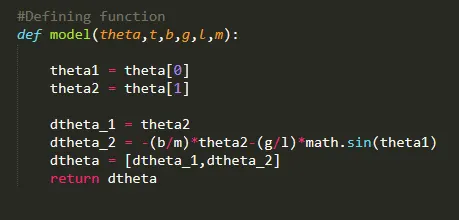
Then a function named model(theta,t,b,g,l,m) was defined that took in parameters theta,t,b,g,l,m.

Then the pendulum parameters were defined.

damping coefficient: 0.05

length of arm: 1m

acceleration due to gravity: 9.81m/s^2

mass of ball: 1kg

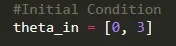
Then the initial conditions were defined:

Initial displacement = 0

Initial angular velocity = 3rad/s

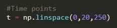
Then the time for which the odeint would solve the differential equations was defined:

The solver would find from 0 to 20s with 250 equally spaced intervals.

Then the ode solver was defined:

theta = odeint(model,theta_in,t,args = (b,g,l,m))

How the solver works:

odeint runs the function model and passes the arguments to the function.

theta_in is passed to theta which is defined in the model arguments.

theta1 = theta[0] corresponds to the displacement values

theta2 = theta[1] corresponds to the velocity values.

odeint then integrates the functions

dtheta_1 = theta2, integrating this function returns theta1(displacement) values.
dtheta_2 = -(b/m)*theta2-(g/l)*math.sin(theta1), integrating this function returns theta2(angular velocity) values.

The values of dtheta_1 and dtheta_2 are found for each time step saved into an array dtheta

return dtheta allows us to retrieve the calculated value from the function.

Function code snippet:

Pendulum animation:

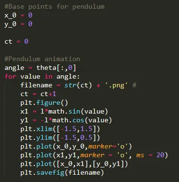
The motion of the pendulum is realized using its displacement values. A variable angle is created to store the displacement values from theta.

Then a for loop is made which runs as many times as the total number of values stored in angle.

a counter variable ct was defined outside the loop, and a file name is created by converting this number to a string. This allows us to store the generated images in the correct order(as time goes from 0 to 20seconds). If the images are not in the correct order then the animation will not be generated correctly.

The bob position was defined using x1 and y1.

x1 = l*math.sin(value), horizontal displacement

y1 = -l*math.cos(value), vertical displacement

The limits for the axes were defined in order to view the pendulum movement correctly.

Then the pendulum base was plotted using x_0 and y_0 values and marker='o' was used to plot a circle.

plt.plot(x_0,y_0,marker='o')

The pendulum bob was plotted using x1 and y1 and marker='o' was used to plot a circle and marker size was defined using ms = 20.

plt.plot(x1,y1,marker = 'o', ms = 20)

The pendulum string was plotted using base and bob points.

plt.plot([x_0,x1],[y_0,y1])

The figure generated was saved using plt.savefig(filename).

Code Snippet:

Result:

Plot:
The Red line shows the displacement plot and the blue line the angular velocity plot. The damping effect is not clearly visible because the system has a low damping coefficient.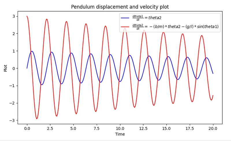

GIF:

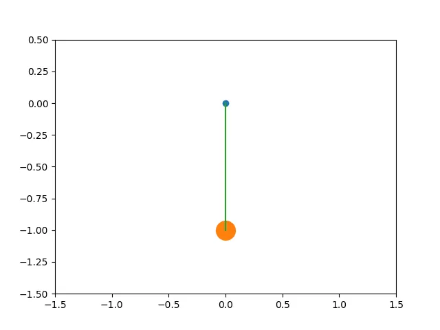
The bob is initially at resting position and an angular velocity of 3rad/s is applied to it.

The motion of the bob can be observed with this animation:

Learning Outcomes:

Through this challenge, I learned

How to break a 2nd order ODE into two first-order ODEs.

How to solve an ODE using odeint in Python.

How to animate the motion of a pendulum bob in Python.