Application of SVM for data classification using Steel Plates Faults Data Set (UCI)
SVM: Support Vector Machines is a classification algorithm.
Working:
Scatter plot of petal length vs petal width for Iris Setosa(green) and Iris Versicolor(Blue).
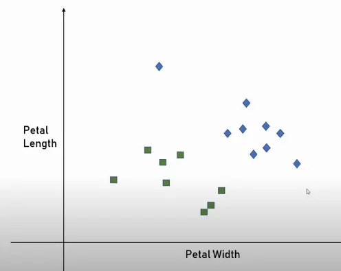
The data can be classified using several different boundary lines. SVM is a method of deciding which boundary line suits the dataset best.
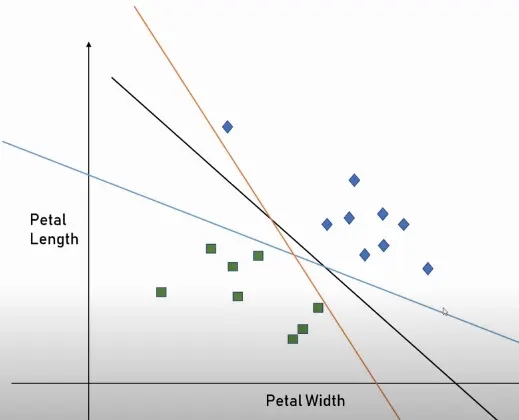
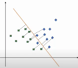
The distance between the closest points(support vectors) to the partitioning line is called the margin. The algorithm will choose the line with the highest margin as the classifier.
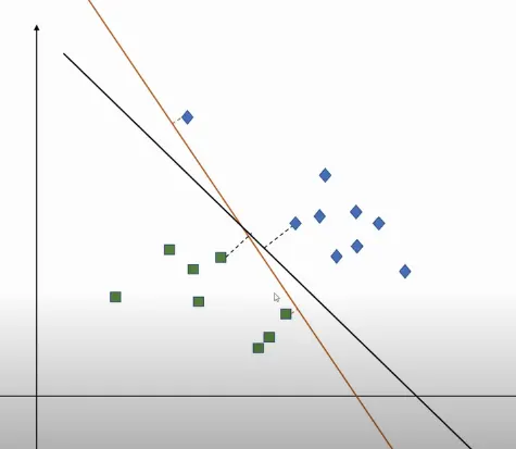
For a model with two features, it is a line, with three it is a plane, however with n dimensions, it becomes difficult to visualize it. However, mathematically for n dimensions, the classifier is called a hyperplane.
Gamma: When deciding the hyperplane, if only the closest points are considered, then the model is said to have high gamma. However, if the further away points are also considered, the model is said to have low gamma. Low gamma modes tend to have accuracy issues but less computation cost.
High gamma:
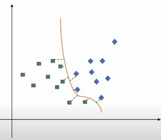
Low gamma:
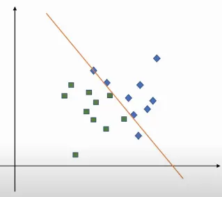
Regularisation: Regularisation refers to how accurately the model should fit the data. A high regularisation can lead to overfitting of the dataset, leading to erroneous predictions. A low regularisation will consist of some misclassified data but will have an overall good accuracy.
High Regularisation:
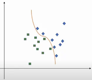
Low regularisation:
Aim: The aim of this challenge is to apply SVM to the "Steel Plates Faults" dataset and evaluate it.
Surface defects in stainless steel plates dataset :
There are 34 fields. The first 27 fields describe some kind of steel plate faults seen in images.
- X_Minimum
- X_Maximum
- Y_Minimum
- Y_Maximum
- Pixels_Areas
- X_Perimeter
- Y_Perimeter
- SumofLuminosity
- MinimumofLuminosity
- MaximumofLuminosity
- LengthofConveyer
- TypeOfSteel_A300
- TypeOfSteel_A400
- SteelPlateThickness
- Edges_Index
- Empty_Index
- Square_Index
- OutsideXIndex
- EdgesXIndex
- EdgesYIndex
- OutsideGlobalIndex
- LogOfAreas
- LogXIndex
- LogYIndex
- Orientation_Index
- Luminosity_Index
- SigmoidOfAreas
The last seven columns are one hot encoded classes, i.e. if the plate fault is classified as "Stains" there will be a 1 in that column and 0's in the other columns. If you are unfamiliar with one-hot encoding, just know that the last seven columns are your class labels.
- Pastry
- Z_Scratch
- K_Scatch
- Stains
- Dirtiness
- Bumps
- Other_Faults
Code:
import pandas as pd
import numpy as np
import matplotlib.pyplot as plt
import seaborn as sns
from sklearn import svm
from sklearn.model_selection import train_test_split
from sklearn.metrics import accuracy_score
from sklearn.metrics import plot_confusion_matrix

#Dataframe df
df = pd.read_csv('faults.csv')
#To print data
print(df)
#To print column names of data
print('n',df.columns)
#To check for datatype and presence of null value for each column
print('n',df.info())
print('n',df.isnull().values.any())

#Last seven columns are type of error classification
label_columns = df.columns.values[-7:]
#Assigning the error classification values to variable targets
targets = (df.iloc[:,-7:]==1).idxmax(1)
print('n',label_columns)
print('n',targets)


#Dropping the 7 error classification columns and retaining only targets
dataset = df.drop(label_columns,axis=1)
#creating a new column 'target' with all classification values
dataset['target']=targets
print('n',dataset)
#Printing count of each type of error
print('n',dataset.target.value_counts())

fig, ax = plt.subplots(1,2,figsize=(15,6))
#Visualising the distribution of each error using histogram and pie chart
sns.countplot(x='target',data=dataset, ax=ax[0])
dataset['target'].value_counts().plot.pie(autopct = '%.1f', ax=ax[1])

#Visualising the correlation among each dataset feature
plt.figure(figsize=(10,11))
sns.heatmap(dataset.corr(),annot=False)

#Dropping features with high correlation to others
dataset=dataset.drop('TypeOfSteel_A400',axis=1)
dataset=dataset.drop('X_Minimum',axis=1)
dataset=dataset.drop('Y_Minimum',axis=1)
print(dataset.shape)


#Assigning feature column values to x
x = dataset.iloc[:,0:24]
#Assingning target column values to y
y = dataset.iloc[:,24]

#Splitting the dataset to training and testing sets
x_train,x_test,y_train,y_test = train_test_split(x,y,test_size = 0.2, random_state = 0)

#Count of each target classification in test set
index = pd.Index(y_test)
print(index.value_counts())

#SVM Model
model = svm.SVC()
model.fit(x_train,y_train)
r = model.fit(x_train,y_train)
Predictions = model.predict(x_test)
print("nSVM accuracy:",accuracy_score(y_test,Predictions))
plot_confusion_matrix(r,x_test,y_test, labels=None, sample_weight=None, normalize=None)

plt.show()
Code Explanation:
The modules needed to execute the program were imported.
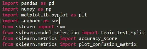
Code Snippet:
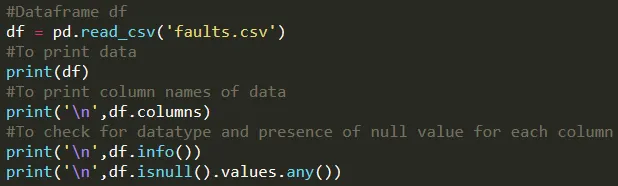
Exploratory data analysis was carried out on the given dataset.
Result:
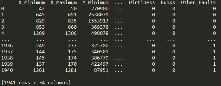
Printing the dataset:
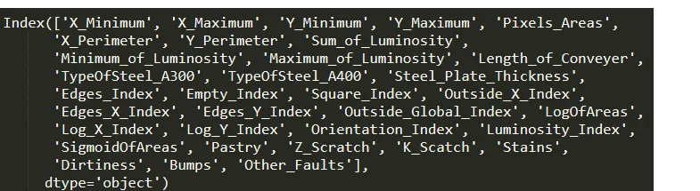
Printing column names:
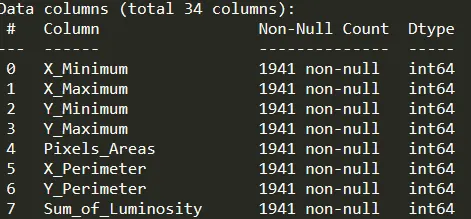
Printing data.info:
Checking for missing data:

Conclusion: The dataset consists of 1941 instances and 34 columns. It does not have any missing data. The results are in one hot-encoded format.
Code Snippet:
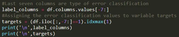
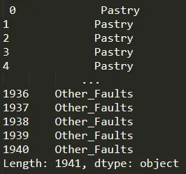
The last 7 columns were target classification. The column names were assigned to label_columns and all the values were indexed using df.iloc and assigned to variable targets.
Result:
Printing label_columns:

Printing targets:
Code Snippet:
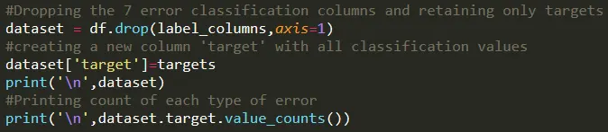
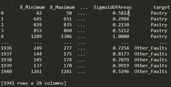
The 7 target columns were then dropped and a new column was created which consisted of all target values.
Result:
Printing new dataset:
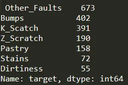
Printing target counts:
Code Snippet:
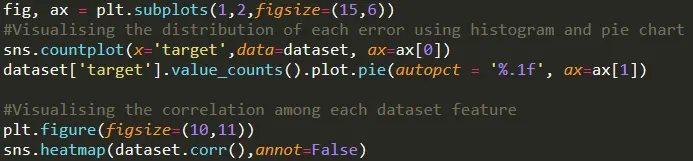
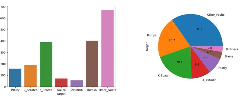
Visualizing the frequency of each target using countplot and plot.pie and the degree of correlation among the features using heatmap.
Result:
Visualising countplot and pieplot:
Heatmap:
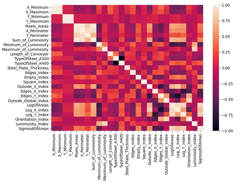
With the help of a heatmap, we can conclude that there is a high correlation between X minimum and X maximum, Y minimum and Y maximum, and type of steel A300 and A400.
Code Snippet:
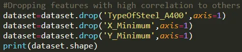
Based on our conclusions from the heatmap, we drop type of steel A400, X minimum and Y minimum.
Result
The shape of the dataset:

There are 1941 instances and 25 columns.
Code Snippet:
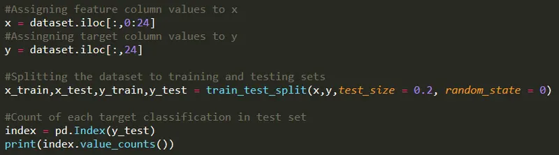
The feature values are assigned to variable x and target values to variable y.
The x and y values are then split into training and testing sets. The test size is 20% of the size of the complete dataset.
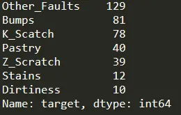
The count of each target in the test set is printed using value_counts().
Result:
Code Snippet:
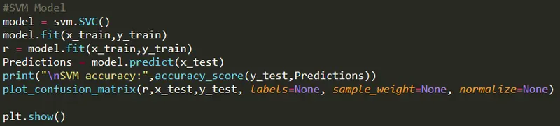
A variable model is created and svm.SVC() model is assigned to it. The svm model is trained with x train and y train values using model.fit. Once the model is trained, the prediction accuracy of the model is observed.
Result:

The SVM model has an accuracy of 48.84%.
Confusion matrix: With the help of the confusion matrix, it is possible to understand which surface defects are being incorrectly classified.
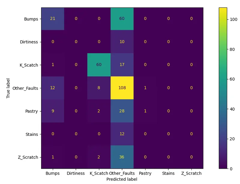
We can observe that majority of the faults are being falsely predicted as other faults. Therefore it is necessary to check the other fault's values.
References: