EDA on Automobile 1985 dataset

Aim: The aim of this challenge is to clean the Automobile 1985 dataset and perform descriptive analytics.

Code:

import numpy as np
import pandas as pd
import matplotlib.pyplot as plt
import seaborn as sns

#To view the entire dataset
pd.set_option("display.max_rows", None, "display.max_columns", None)

df = pd.read_csv('auto.csv')

#Adding column names
df.columns = ['symboling','normalised-losses','make','fuel-type','aspiration','num-of-doors','body-style','drive-wheels','engine-loc','wheelbase','length','width','height','curb-weight','engine-type','no._cyl','engine_size','fuel-sys','bore','stroke','compression','hp','peak-rpm','city-mpg','highway-mpg','price']

#Printing the original dataset
print(df)

print('Original dataset shape and information = ',df.shape)
print(df.info())

#Removing instances in dataset with '?'
for c in df.columns:
	df = df[df[c] != '?']


print(df.info())

#Changing type from object to float
feat = ['normalised-losses','bore','stroke','hp','peak-rpm','price']
for f in feat:
	df[f] = df[f].astype(float)

print('New dataset shape = ',df.shape)
print(df.info())

print(df['make'].value_counts(ascending=True))

#Manufacturer count plot
plt.figure(figsize=(10,5))
sns.countplot(x=df['make'])
plt.xticks(rotation='vertical')
plt.title('Manufacturer count plot')

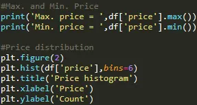
#Max. and Min. Price
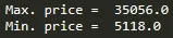
print('Max. price = ',df['price'].max())
print('Min. price = ',df['price'].min())

#Price distribution
plt.figure(2)
plt.hist(df['price'],bins=6)
plt.title('Price histogram')
plt.xlabel('Price')
plt.ylabel('Count')

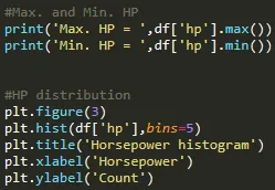
#Max. and Min. HP
print('Max. HP = ',df['hp'].max())
print('Min. HP = ',df['hp'].min())


#HP distribution
plt.figure(3)
plt.hist(df['hp'],bins=5)
plt.title('Horsepower histogram')
plt.xlabel('Horsepower')
plt.ylabel('Count')

print(df)

#Visualising Correlation between features
plt.figure(figsize=(15, 15))
ax = sns.heatmap(df.corr(), annot=True)
plt.title('Correlation between features in dataset')


print('Engine location types = ',df['engine-loc'].unique())

cat = ['fuel-type', 'aspiration', 'num-of-doors', 'body-style','drive-wheels', 'engine-type', 'no._cyl', 'fuel-sys']
fig, axs = plt.subplots(nrows=2, ncols=4, figsize=(10, 10))
for col, ax in zip(cat[0:], axs.ravel()):
	sns.countplot(x=col, data=df, ax=ax)
	plt.xticks(rotation='vertical')

#sns.scatterplot(df['city-mpg'],df['price'])
fig, ax = plt.subplots(2, figsize=(10, 6))
ax[0].scatter(x = df['city-mpg'], y = df['hp'])
ax[0].set_xlabel("city-mpg")
ax[0].set_ylabel("hp")

ax[1].scatter(x = df['city-mpg'], y = df['highway-mpg'])
ax[1].set_xlabel("city-mpg ")
ax[1].set_ylabel("highway-mpg")

plt.show()

"""
from sklearn.preprocessing import LabelEncoder, OneHotEncoder
labelencoder = LabelEncoder()
ohe = OneHotEncoder()
feat = ['num-of-doors','body-style','drive-wheels','no._cyl','fuel-sys','engine-type']
for f in feat:
	df[f] = labelencoder.fit_transform(df[f])
	#df = pd.get_dummies(df[f], prefix=f)

	#enc_df = ohe.fit_transform(df[[]])
print(df)
#df['Cat'] = labelencoder.fit_transform(bridge_df[feat])
"""

Data cleaning:

On visualizing the initial dataset, we can see that

Features:

1. symboling: [its assigned insurance risk rating -> [-3, -2, -1, 0, 1, 2, 3]]
2. normalized-losses: [average loss payment per insured vehicle year -> continuous from 65 to 256.]
3. make: [ Manufacturer name eg : alfa-romero, audi, bmw, chevrolet, dodge, honda,isuzu etc. ]
4. fuel-type: [diesel, gas]
5. aspiration: [std, turbo]
6. num-of-doors: [four, two].
7. body-style: [hardtop, wagon, sedan, hatchback, convertible]
8. drive-wheels: [4wd, fwd, rwd]
9. engine-location: [front, rear]
10. wheel-base: [continuous from 86.6 120.9]
11. length: [continuous from 141.1 to 208.1]
12. width: [continuous from 60.3 to 72.3]
13. height: [continuous from 47.8 to 59.8]
14. curb-weight: [continuous from 1488 to 4066]
15. engine-type: [dohc, dohcv, l, ohc, ohcf, ohcv, rotor]
16. num-of-cylinders: [eight, five, four, six, three, twelve, two]
17. engine-size: [continuous from 61 to 326]
18. fuel-system: [1bbl, 2bbl, 4bbl, idi, mfi, mpfi, spdi, spfi]
19. bore: [continuous from 2.54 to 3.94]
20. stroke: [continuous from 2.07 to 4.17]
21. compression-ratio: [continuous from 7 to 23]
22. horsepower: [continuous from 48 to 288]
23. peak-rpm: [continuous from 4150 to 6600]
24. city-mpg: [continuous from 13 to 49]
25. highway-mpg: [continuous from 16 to 54]

Output Variable price: [continuous from 5118 to 45400]

Original dataset size:

Code:

Output:

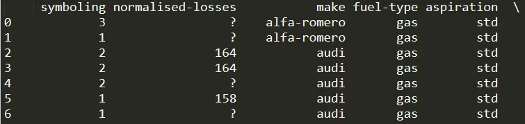
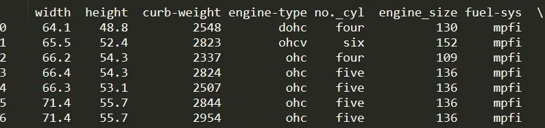
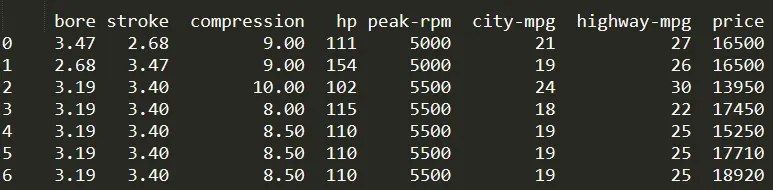
The original dataset consists of 204 instances and 26 columns.

Original dataset info:

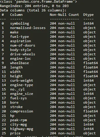
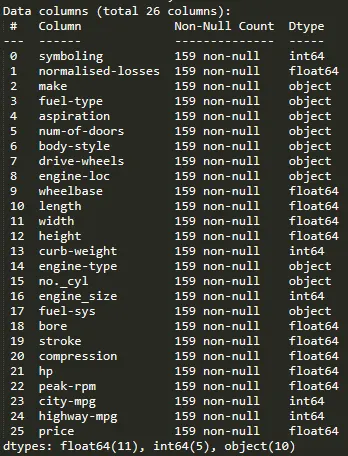
When checking the data info we see that 'normalised-losses','bore','stroke','hp','peak-rpm', and 'price' are of datatype object even though they contain numeric values.

This is because they contain '?' where ever there is data missing. We then clean the data by removing those instances.

Data cleaning:

Code:

The shape of the dataset has now reduced from 204 instances to 159.

Converting datatype from object to float for 'normalised-losses','bore','stroke','hp','peak-rpm', and 'price'

Code:

Output:

Descriptive analytics:

Manufacturer count:

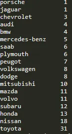
To see the distribution of each make, we print the count of each value.

Code:

Output:

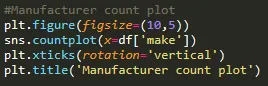
We then visualize it using sns.countplot:

Code:

Output:

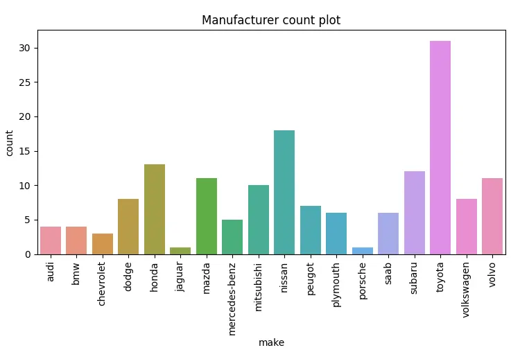
From the above graph, we observe that the maximum number of cars in the dataset are from Toyota and the lowest from Porsche.

Price histogram:

Code:

Output:

Code Explanation:

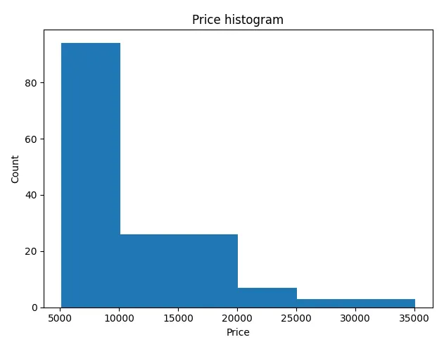
For creating price histogram, we set bins=6. This creates 6 categories from the lowest price 5118 up to the highest price 35056. We can observe that majority of the cars are between 5000-10000 dollars.

Horsepower histogram:

Code:

Output:

Code Explanation:

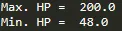
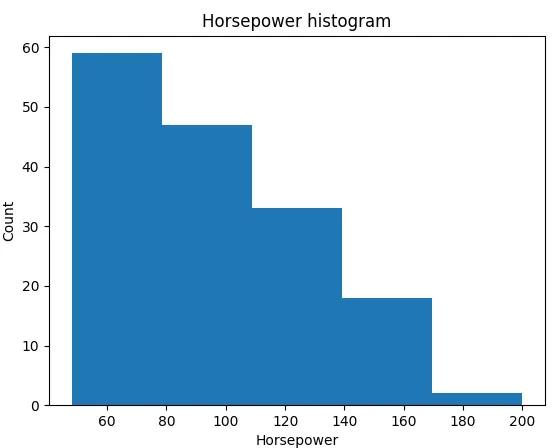
For creating a horsepower histogram, we set bins=5. This creates 5categories from the lowest horsepower 48 up to the highest horsepower 200. We can observe that majority of the cars are between 48-80 horsepower.

Correlation between the features: We check for the degree of correlation between the features present in the dataset using sns.heatmap. It is good practice to drop highly correlated factors since keeping them can lead to erroneous results.

Code:

Output:

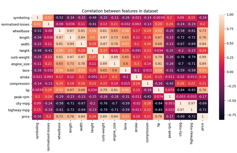
There is a high degree of correlation between curb-weight and width, length, engine size, and horsepower and between city-mpg and highway-mpg.

Count of each value present in 'fuel-type', 'aspiration', 'num-of-doors', 'body-style','drive-wheels', 'engine-type', 'no._cyl', and 'fuel-sys'.

Code:

Result:

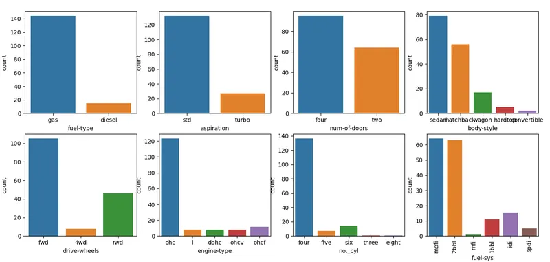
We observe that majority of the vehicles are naturally aspirated, four-door, front-wheel drive, with a four-cylinder engine and run on gas.

Also, the majority of the cars are sedan whereas the least are convertible body type.

References:

https://www.kaggle.com/ashishpal2702/1985-auto-imports-database-analyses-prediction