Genetic Algorithm

AIM: The aim of this project is to optimize the Stalagmite function and find the global maxima of the function using the ga() function in MATLAB.

GOVERNING EQUATIONS:

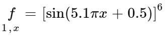
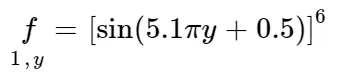
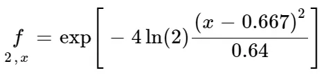
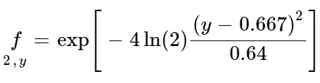
, is the stalagmite function

OBJECTIVES:

The objective of this challenge was to optimize the stalagmite function using and find the global maximum using the ga() function.

The ga() function is used in finding the minimum of a function using a genetic algorithm based on Charles Darwin's theory of evolution.

CODE EXPLANATION:

ga(), is a function defined in the MATLAB database that returns the minimum of a function using genetic algorithm. It takes the function as input, and a number n, which defines the number of variables of the function.

In order to obtain the maximum value, the Minus sign was added to the stalagmite function. This way the maximum value would now become the least value and would be returned by the function.

[inputs,fval] returns the coordinates and the least value of the function.

The main program is calling two subprograms, get_stalagmite, and stalagmite. The get_stalagmite function is being called in order to create the stalagmite surface plot. It is taking two inputs and is used to create the reference plot. The stalagmite function is being called by the ga() function and is taking only one input. It cannot take more than one input since the ga() syntax restricts it.

The genetic algorithm uses concepts from evolutionary biology and creates solution points from the initial data set, and using the solution points creates a subsequent generation of points using Selection, Crossover, and Mutation.

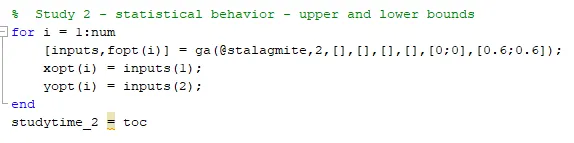
is the syntax of the ga() function and [0;0] defines the lower bound and [0.6;0.6] defines the upper bound for the function. Since no linear equalities A,b, and inequalities Aeq and beq exits, they are defined as [] in the function definition.

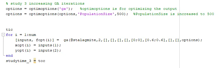
For study 3, the population size was increased. This allowed us to get the solution for the global maximum value of the function. optimoptions() function was used to define the population size as 500. By increasing the population size, the computation time also increased. options was then defined in the ga() function definition.

CODE:

clear all
close all
clc

% Defining our search space
x = linspace(0,0.6,150);
y = linspace(0,0.6,150);

num = 50;
 
f = get_stalagmite(x,y);

tic
% study 1
for i = 1:num
       [inputs, fopt(i)] = ga(@stalagmite, 2);
        xopt(i) = inputs(1);
        yopt(i) = inputs(2);
end
studytime_1 = toc 

figure(1)
subplot(2,1,1)
surfc(x, y , f)
xlabel('x value')
ylabel('y value')
zlabel('function value')
shading interp
hold on 
plot3(xopt,yopt,abs(fopt),'marker','o','markersize',5,'markerfacecolor', [ 0.5 0.5 0.5])
title('Case 1: Unbound Inputs')

subplot(2,1,2)
plot(abs(fopt))
xlabel('Iterations')
ylabel('Functions maximum')

num = 50;
tic
%  Study 2 - statistical behavior - upper and lower bounds
for i = 1:num
    [inputs,fopt(i)] = ga(@stalagmite,2,[],[],[],[],[0;0],[0.6;0.6]);
    xopt(i) = inputs(1);
    yopt(i) = inputs(2);
end
studytime_2 = toc


figure(2)
subplot(2,1,1)
hold on
surfc(x, y ,f)
xlabel('x value')
ylabel('y value')
zlabel('function value')
shading interp
plot3(xopt,yopt,abs(fopt),'marker','o','markersize',5,'markerfacecolor',[0.5,0.5,0.5])
title('Case 2: Bounded inputs')
subplot(2,1,2)
plot(abs(fopt))
xlabel('Iterations')
ylabel('Function maximum')
shading interp

[inputs, fval] = ga(@stalagmite,2);

% study 3 increasing GA iterations
options = optimoptions('ga');   %optimoptions is for optimizing the output
options = optimoptions(options,'PopulationSize',500);  %PopulationSize is increased to 500 


tic 
for i = 1:num
    [inputs, fopt(i)] =  ga(@stalagmite,2,[],[],[],[],[0;0],[0.6;0.6],[],[],options);
    xopt(i) = inputs(1);
    yopt(i) = inputs(2);
end
studytime_3 = toc

figure(3)
subplot(2,1,1)
hold on
surfc(x, y ,f)
xlabel('x value')
ylabel('y value')
zlabel('function value')
shading interp
plot3(xopt,yopt,abs(fopt),'marker','o','markersize',5,'markerfacecolor',[0.5,0.5,0.5])
title('Case 3: Bounded inputs with increase in population size')
subplot(2,1,2)
plot(abs(fopt))
xlabel('Iterations')
ylabel('Function maximum')
shading interp
[inputs, fval] = ga(@stalagmite,2);

function [s] = get_stalagmite(x,y)
  

 [xx yy] = meshgrid(x,y);
  

  x1 = (sin(5.1*pi*xx+0.5)).^6;
  
  y1 = exp((-4*log(2)*(((xx-0.0667).^2)./0.64)));

  x2 = (sin(5.1*pi*yy+0.5)).^6;
  
  y2 = exp((-4*log(2)*(((yy-0.0667).^2)./0.64)));
  
  s = x1.*x2.*y1.*y2;
 


end

function [s] = stalagmite(input_vector)

  a = input_vector(1);
  b = input_vector(2);
  
  x1 =    (sin(5.1*pi*a+0.5))^6;
  
  y1 =   exp((-4*log(2)*(((a-0.0667)^2)/0.64)));

  x2 =   (sin(5.1*pi*b+0.5))^6;
  
  y2 = exp((-4*log(2)*(((b-0.0667)^2)/0.64)));
  
  s = -x1*x2*y1*y2;
end

CODE OUTPUT:

Case 1:

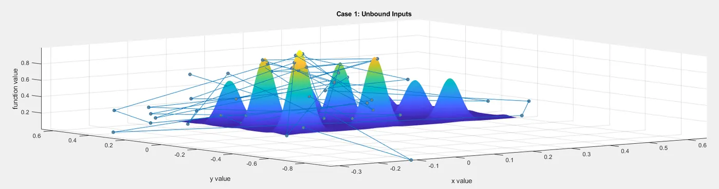
The above plot represents the stalagmite function surface model and the solutions for the function that were obtained by ga() function without any bounds. The points are spread across the whole area and fail to give a proper solution.

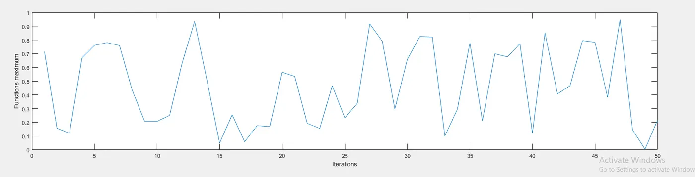
The function maximum value vs the number of iterations shows how the solution varies across a wide range when the loop is run 50 times. This is a poor result and is not of any use.

Case 2: ga() with bounded inputs

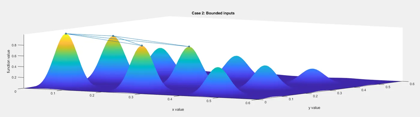
The above plot shows that the maximum value lies between the 4 points plotted on top of the peaks. The solution is much clearer because of the domain constraints.

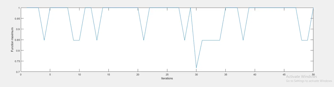
The variation in the solution with each iteration is reduced to a great extent.

Case 3: ga() with bounded inputs with an increase in population size

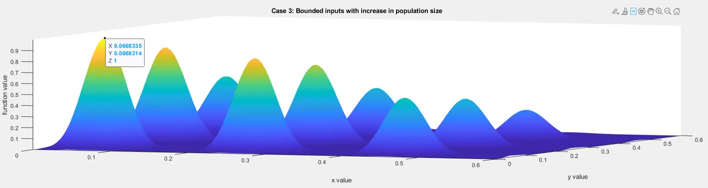
The marker highlights the point at which the ga() function predicts that the solution of the stalagmite function is maximum.

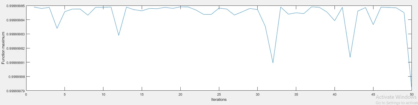
The above plot represents the variation of the ga() output, and the changes in the predicted solution are almost negligible.

REFERENCES:

https://www.youtube.com/watch?v=1i8muvzZkPw&ab_channel=MATLAB