Solving second order ODEs using MATLAB

AIM: The aim of this challenge is to simulate the motion of a pendulam using a second order differential equation in MATLAB.

GOVERNING EQUATIONS:

where,

g is acceleration due to gravity

b is damping constant

m is mass of the bob

l is the length of the string

θ is the angular displacement

OBJECTIVES:

The main objective of this project is to

1. Plot Displacement, Velocity vs Time graph

2. Animate how the pendulum would oscillate using MATLAB

CODE LOGIC:

The initial conditions were defined first, and the initial displacement and velocity were assigned to a variable 'theta0' as a coloumn matrix, since ode45 would accept only coloumn matrix as a valid input.

Time interval was specified as 0 to 20 seconds and linspace() function was used to split the duration to 200 parts in order to generate a smoother curve.

To solve the ODE, ode45 is a MATLAB function which integrates the differential function with the intial conditions specified. The numerical method used to solve the function is the Runge-Kutta Method. ode45 takes 3 inputs, first the ODE to be integrated, second the time span and then the displacement condition. It is important that the variables be entered in the same order for the program to generate the desired set of results.

The second order differential equation was split into two first order equations.

The main called the ODE which was defined in a another program, which had equations of the first order in the form of a coloumn matrix.

The results obtained from the function were stored onto two variables, which were then plotted.

Legend command was used to highlight the displacement and velocity curve, for clear understanding of the generated plot.

CODE:

clear all
close all
clc


l = 1;
m = 1;
b = 0.05;
g = 9.81;


  %Initial condition
  theta0 = [0;3];

  %time points 
  t_span = linspace(0,20,200);

  %solve ODE
  [t,results] = ode45(@(t,theta)ode_func(t,theta,l,b,m,g),t_span,theta0);

    figure(1)
    plot(t,results(:,1))
    hold on 
    plot(t,results(:,2))
    xlabel('Time')
    ylabel('Plot')
    lgd = legend('Displacement','Velocity')
    lgd.FontSize = 8
    
    xo = 0;
    yo = 0;
    ct = 1;
    for i = 1:length(results)
        figure(2)
        ang = results(:,1);
        x =  l*sin(ang(i));
        y = -l*cos(ang(i));
        plot([xo x],[yo y],'LineWidth',2,'Marker','s','MarkerSize',28,'MarkerFaceColor','b','MarkerIndices',1)
        hold on
        plot(x,y,'Marker','o','MarkerSize',30,'MarkerFaceColor','r')      
        axis([-1 1 -1.5 0.5])
        grid on
        pause(0.1)
        M(ct) = getframe(gcf);
        ct = ct+1;
       hold off
    end
    
movie(M)
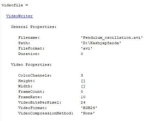
videofile = VideoWriter('Pendulum_oscillation', 'uncompressed AVI');
videofile.FrameRate = 10
open(videofile)
writeVideo(videofile,M)
close(videofile)

  

function [dtheta_dt] = ode_func(t,theta,l,b,m,g)

    theta1 = theta(1)
    theta2 = theta(2)
    dtheta1_dt = theta2;
    dtheta2_dt = -(b/m)*theta2 - (g/l)*sin(theta1);
    dtheta_dt = [dtheta1_dt; dtheta2_dt];
end

OUTPUT:

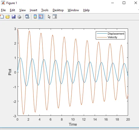
The above graph was obtained using plot() command, using the results obtained by the ode45 function. Results was a 200x2 matrix, and the angular displacement was defined in the first coloumn and velocity in the second coloumn. Therefore in order to obtain only the displacement for plotting the graph, results(:,1) was used. This way, all elements belonging to the first matrix could be indexed. Similarly results(:,2) was used to index the velocity values.

Drive link:

https://drive.google.com/file/d/1PTcLyn8DeWBREf5Hc6vxuUVWIMK6afO1/view?usp=sharing

The video was created using a 'for' loop, where the loop would run for as many times as the number of results obtained. For each iteration of the for loop, the end point of the string would move by length*sin(angular displacement) along x direction and length*cos(angular displacement) along y direction. Marker tool was used to add the circle at the end end of the string and a square at the fixed end of the string.

Variable ct was used as a counter for each frame. Movie and VideoWriter command was used to display each frame as a movie, and to save the movie in the desired format. Open() command was used to open a file and writeVideo() was used to write the video into the file. Care was taken to make sure the correct case was used for each function, since MATLAB is case sensitive for built in functions and variables, and close() was used to close the file.