Week 5 Sphere pressing on a plate
Sphere Pressing on a Plate Simulation Using
ANSYS Workbench 2020 R2
Thejan Sasilal
OBJECTIVES
For this challenge, perform the analysis to simulate a sphere pressing on a plate.
Use Structural steel for both sphere and plate but the material of the plate must be Non Linear.
Press the sphere onto plate 4mm downwards and retract it. The plastic deformation must be captured by you. Attach appropriate images and make a detailed report.
- INTRODUCTION
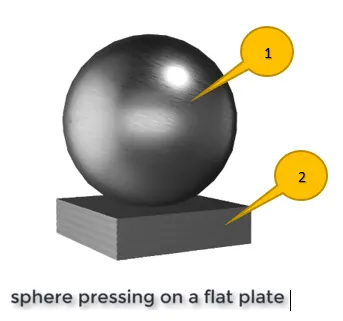
In this challenge, we are simulating a sphere is pressing over a flat plate to find out the plastic deformation of flat plate.
- DESIGN SPECIFICATION
Assigned the following materials for each geometry from engineering data.
Material Assignment:
Sphere: Structural Steel
Plate: Structural Steel NL
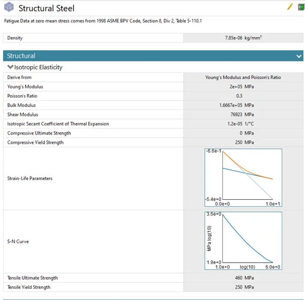
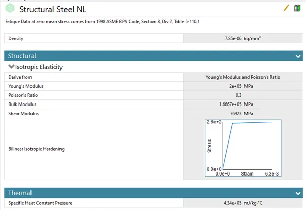
Imported the geometry and open it in Space Claim and check.
- STATIC ANALYSIS
Open Mechanical modeller for analysis.
Consider all units are in metric.
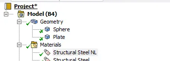
Rename geometry as Sphere, Plate
4.1 CONNECTIONS
|
Contact is said to occur when the surfaces of two separate objects touch each other such that the surfaces are mutually tangent to each other. The surfaces in contact do not interpenetrate and can transmit forces from one body to the other. In order to prevent the interpenetration between the surfaces, the ANSYS program or any FEA software has to establish relations between the surfaces and this is done using CONTACT FORMULATIONS. When penetration is prevented by the program, it is said to have enforced Contact Compatibility. When the program fails to enforce contact compatibility between two surfaces in contact, interpenetration occurs to a large extent and the solver will face convergence issues and be forced to stop. |
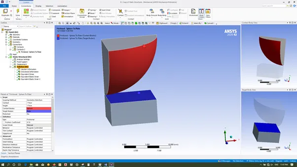
Delete the default contact generated by Ansys. Insert manual contact region.
|
In an interface, we define the contact and target. While deciding between these two, we should keep in mind that ANSYS considers the contact body as the one which is not allowed to penetrate into the target body. But the target is allowed to penetrate into the contact body. If you are unsure of the behaviour of your system, then you can choose Symmetric type of contact. Otherwise, an Asymmetric type of contact can be used. |
- Select following as Contact & Target
- Contact: Sphere face
- Target: Top face of plate
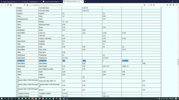
- https://roymech.org/Useful_Tables/Tribology/co_of_frict.html from this link find the coefficient of friction of the contact materials.
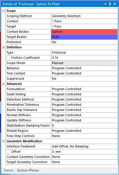
Consider the following settings for contact.
|
Frictional: We can specify any non-negative value as the frictional coefficient. So, the contact will handle shear stresses up to what is specified by the frictional coefficient. After this value, sliding will start to take place. |
4.2 MESH CREATION
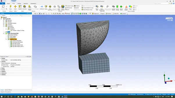
Generate default meshing
4.3 ANALYSIS SETTINGS
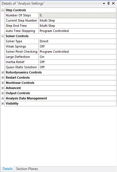
Consider following as the analysis settings for all steps.
|
STEP CONTROLS Time is an essential parameter in tracking all the analysis even though the model is time-dependent or not. In a static analysis where it is time-independent, the analysis takes place as steps in which the steps are incremented linearly. The beginning time will be 0, and the time for the final load application is 1. If some more load is added, then the time is going to be 2. Here, the time is not considered as minutes or seconds but as a counter or tracker. The sub steps respective to the load steps will vary linearly. Large deflection This option helps the solver whether the large deflection, large stain, large rotation happening in the simulation should be taken into account. It is available for static structural and transient structural analysis. Enabling this by ON will help the solver to consider the large strain happening, such as metal forming in a simulation and deflection. SOLVER CONTROLS Solver controls provide some properties based on the analysis type. For both the static structural analysis and transient structural analysis the common properties are ● Solver type ● Weak springs ● Large deflection Solver type Helps in choosing the required solver type for carrying out a simulation. It offers three options, Program controlled: default option. The program automatically chooses the solver based on the model application. Direct: This is one of the solver types where the solver uses a Sparse solver (solver handles a system of equations where the coefficient matrix entries contain mostly zero) to solve the model. Iterative: This type, when chosen, solves the model in PCG (Preconditioned Conjugate Gradient) or ICCG (Incomplete Cholesky Conjugate Gradient) solver. This is mainly used for electric and electromagnetic simulations. |
4.4 BOUNDARY CONDITIONS
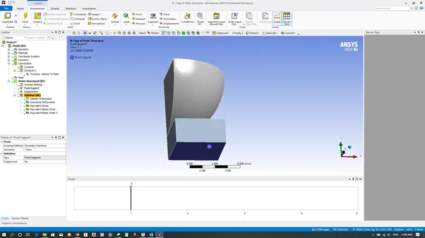
1) Right click Static Structural & Insert Fixed Support. Select bottom face of the plate.
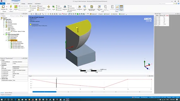
2) Right click Static Structural & Insert Displacement. Select top face of sphere as geometry. Select tabular data for Y-Component.
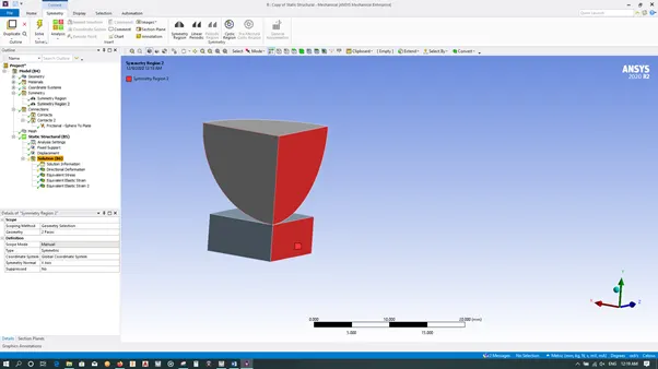
4.5 SYMMETRY REGION
Click on the Model and select Symmetry Region from the toolbar.
1) Select side faces of Sphere & Plate
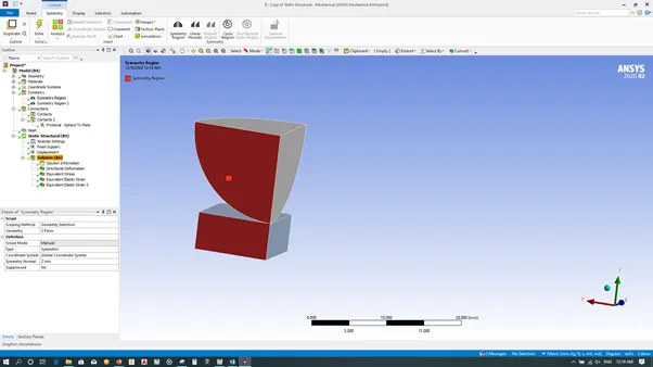
2) Select other side faces of Sphere & Plate
4.6 SOLUTIONS
|
|
Result |
Findings |
|
Directional Deformation about Y- axis |
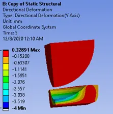 |
4 mm displacement of Sphere is visible from the simulation |
|
Equivalent Stress on Plate |
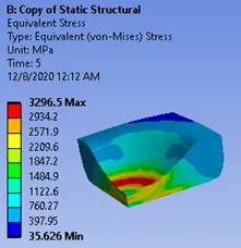 |
Maximum stress developed in the plate is 3296.5 MPa, and it is higher than the young’s modulus (250 MPa) of structural steel NL. As the stress developed is higher than the young’s modulus, the plate got plastically deformed. |
|
Equivalent Elastic Strain |
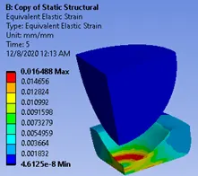 |
Since the center portion of the plate is deforms more, here the strain developed is more. |
|
Equivalent Elastic Strain on Sphere |
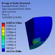 |
The maximum stain developed in the sphere is near to the periphery. |
- CONCLUSSION
Simulation of sphere pressing flat plate process conducted with structural steel as sphere material and structural steel NL as plate material. From the analysis it is found that beyond the elastic limit the material remains in the plastic state, even after removal of load.