Week 4 -Wire Bending Challenge
Wire Bending Challenge Simulation Using
ANSYS Workbench 2020 R2
Thejan Sasilal
OBJECTIVES
For this challenge, you will have to perform an analysis to simulate the bending of a wire in ANSYS. You will have to use Copper Alloy (Non Linear), Aluminium Alloy (Non Linear) and Magnesium Alloy (Non Linear) for the wire alone. You need to find out the Equivalent stress and Equivalent strain on the wire alone. Compare the results and submit a well formatted report on this
- INTRODUCTION
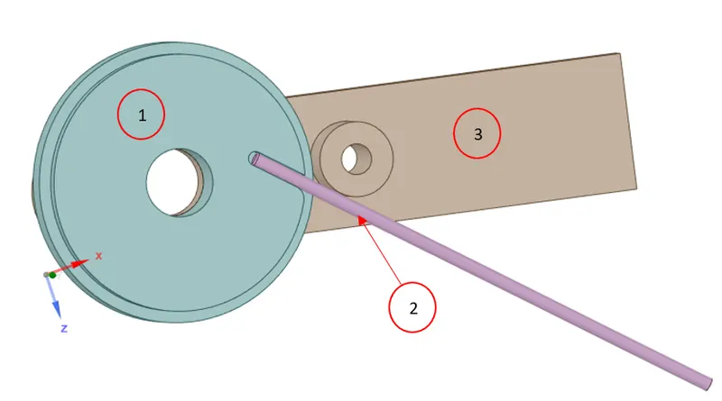
The work piece consisting of a metal wire [2] is fed through the die (wheel) [1] adapted with bending slot suited for the bending shapes. The rotary bending tool (Lever) [3] bends the wire around the die resulting in plastic deformation.
In this challenge, we are considering 3 different materials for wire and comparing results in different conditions.
- DESIGN SPECIFICATION
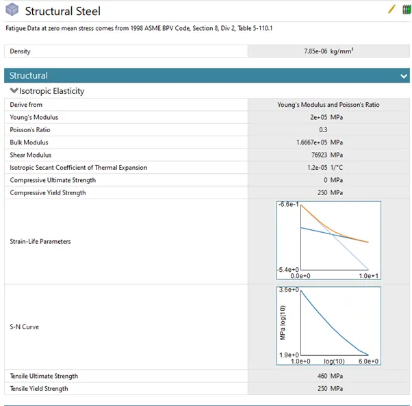
Assigned the following materials for each geometry from engineering data.
Material Assignment:
Wire: Copper Alloy NL / Aluminium Alloy NL / Magnesium Alloy NL
Wheel & Lever: Structural Steel
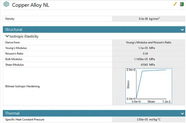
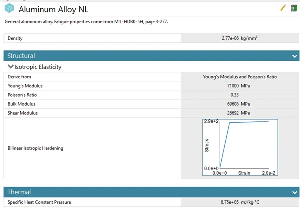
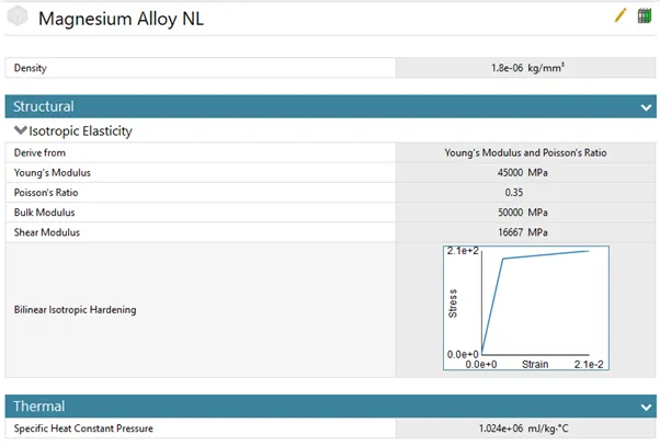
Imported the geometry and open it in Space Claim and check.
- STATIC ANALYSIS
Open Mechanical modeller for analysis.
Consider all units are in metric.
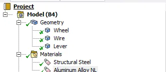
Rename geometry as Wheel, Wire & Lever
4.1 CONNECTIONS
|
Contact is said to occur when the surfaces of two separate objects touch each other such that the surfaces are mutually tangent to each other. The surfaces in contact do not interpenetrate and can transmit forces from one body to the other. In order to prevent the interpenetration between the surfaces, the ANSYS program or any FEA software has to establish relations between the surfaces and this is done using CONTACT FORMULATIONS. When penetration is prevented by the program, it is said to have enforced Contact Compatibility. When the program fails to enforce contact compatibility between two surfaces in contact, interpenetration occurs to a large extent and the solver will face convergence issues and be forced to stop. |
Delete first two default contacts generated by Ansys.
|
In an interface, we define the contact and target. While deciding between these two, we should keep in mind that ANSYS considers the contact body as the one which is not allowed to penetrate into the target body. But the target is allowed to penetrate into the contact body. If you are unsure of the behaviour of your system, then you can choose Symmetric type of contact. Otherwise, an Asymmetric type of contact can be used. |
- Select following as Contact & Target
- Contact: Outer faces of wire
- Target: Outer face of lever pin
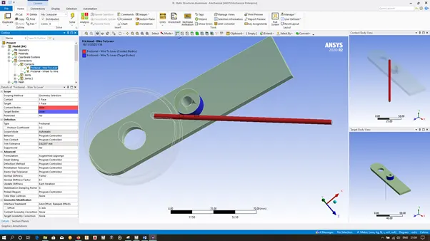
- Create duplicate of the first contact and flip Contact/ Target, select following as Contact & Target
- Contact: Side faces of wheel grove (4 no’s)
- Target: Outer face of wire (1 no)
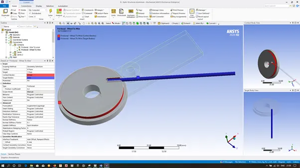
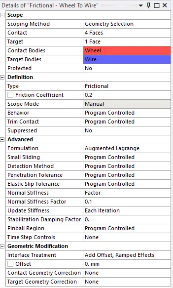
Select both contacts & consider the following settings
|
Frictional: We can specify any non-negative value as the frictional coefficient. So, the contact will handle shear stresses up to what is specified by the frictional coefficient. After this value, sliding will start to take place. Augmented Lagrange: This method is also a penalty-based method. It uses the same equation for solving but has an extra augmentation constant, λ. Because there is an extra term in the equation, the contact force becomes less sensitive to the stiffness. So, there will be lesser penetration at the contacts. Hence, this formulation is preferred more. 𝑭𝒏𝒐𝒓𝒎𝒂𝒍= 𝒌𝒏𝒐𝒓𝒎𝒂𝒍× 𝒙𝒑𝒆𝒏𝒆𝒕𝒓𝒂𝒕𝒊𝒐𝒏+ 𝝀 If penetration present is large, the solver will require additional iterations to converge. Contact penetration is allowed in this formulation but it is more controlled than it was in pure penalty method. This method can be used with any type of contact NORMAL STIFFNESS Normal stiffness helps in controlling the amount of penetration between the contact and target surfaces. Normal stiffness value/factor directly helps in the convergence of the solution. If the stiffness value is small, there would be a large amount of penetration, although it is helpful in converging. If the value is large, there won’t be any penetration of the surfaces, but it results in convergence issues. Hence, it is important that a nominal value should be chosen. It provides some options. They are, Program controlled: This is a default setting. The program takes the normal stiffness value/factor. Factor: The normal ‘normal stiffness factor’ range is from 0.01-10. The reasonable value for bonded contacts is chosen as 10, and for other contact types, it is chosen as 1.0 for bulk deformation. If there is a bending deformation, a value of 0.1 can be chosen, but we must be careful that the smaller values of deformation can cause penetration. Value: Here, the stiffness value is provided manually by the user. The value mentioned should be a non-zero positive value. INTERFACE TREATMENT The interface treatment option helps us to define how the contact surface should be treated. It is enabled only when the contact type is set to frictionless, rough, or frictional. Add offset, Ramped effects: Offset is nothing but adding an extra user-inputted distance. Adding offset helps in bringing the two bodies into initial contact with the loading values ramped at the first load step. Enabling this option enables the offset option, which helps the user to enter the value manually. Positive value brings the body closer, and the negative value moves the body apart. |
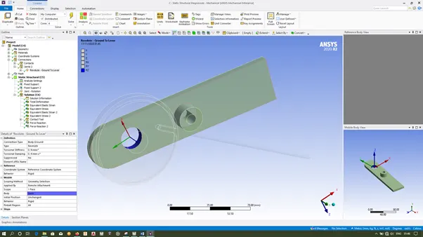
- Insert revolute joint, select inner face of lever.
4.2 MESH CREATION
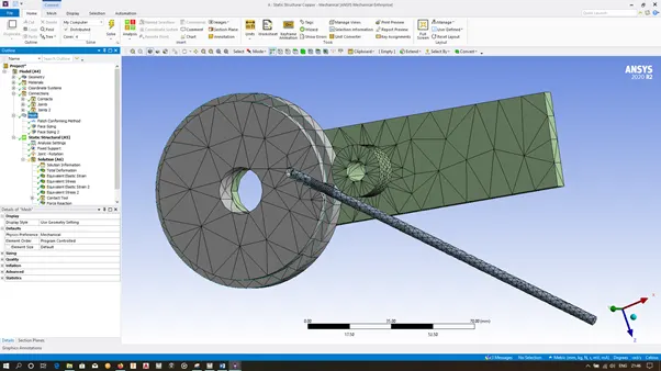
1) Insert Method, select all three geometries. Select method as tetrahedrons.
2) Insert Sizing, select bend face, outer face & fillet face of wire, outer face of lever pin. Input element size of 2.2mm.
3) Click the wheel bend surface & create coordinate system. Select the created coordinate system and select x offset and z offset. Input 3mm & -3mm respectively for x offset and z offset respectively.
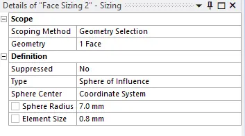
Insert Sizing, select wire outer face and follow the below settings.
4.3 ANALYSIS SETTINGS
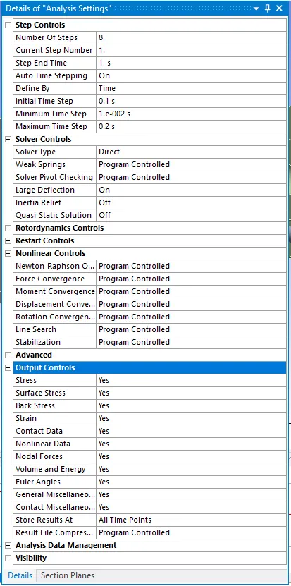
1) Consider following as the analysis settings for 1st step.
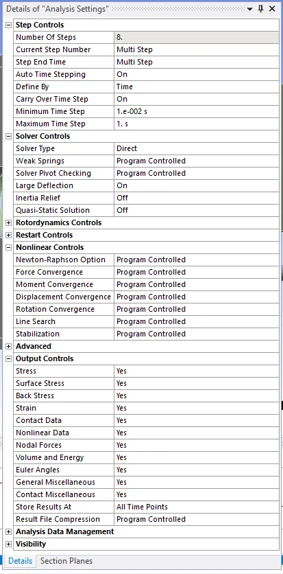
2) Consider following as the analysis settings for 2nd to 8th step.
|
STEP CONTROLS Time is an essential parameter in tracking all the analysis even though the model is time-dependent or not. In a static analysis where it is time-independent, the analysis takes place as steps in which the steps are incremented linearly. The beginning time will be 0, and the time for the final load application is 1. If some more load is added, then the time is going to be 2. Here, the time is not considered as minutes or seconds but as a counter or tracker. The sub steps respective to the load steps will vary linearly. Large deflection This option helps the solver whether the large deflection, large stain, large rotation happening in the simulation should be taken into account. It is available for static structural and transient structural analysis. Enabling this by ON will help the solver to consider the large strain happening, such as metal forming in a simulation and deflection. SOLVER CONTROLS Solver controls provide some properties based on the analysis type. For both the static structural analysis and transient structural analysis the common properties are ● Solver type ● Weak springs ● Large deflection Solver type Helps in choosing the required solver type for carrying out a simulation. It offers three options, Program controlled: default option. The program automatically chooses the solver based on the model application. Direct: This is one of the solver types where the solver uses a Sparse solver (solver handles a system of equations where the coefficient matrix entries contain mostly zero) to solve the model. Iterative: This type, when chosen, solves the model in PCG (Preconditioned Conjugate Gradient) or ICCG (Incomplete Cholesky Conjugate Gradient) solver. This is mainly used for electric and electromagnetic simulations. NONLINEAR CONTROLS Nonlinear control provides some properties based on their analysis systems. Here, the nonlinear controls for the steady-state, static, and transient structural analyses are discussed. |
4.4 BOUNDARY CONDITIONS
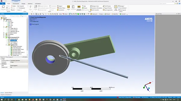
1) Right click Static Structural & Insert Fixed Support. Select inner face of wheel.
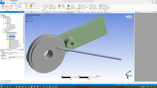
2) Right click Static Structural & Insert Fixed Support. Select face of wire.
3) Right click Static Structural & Insert Joint Load. Select inner face of Lever and input the values.
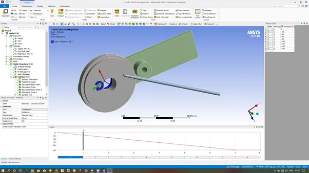
4.6 SOLUTIONS
|
|
Copper Alloy NL |
Aluminium Alloy NL |
Magnesium Alloy NL |
Comparison |
|
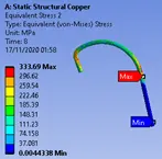
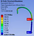
Equivalent stress – Wire |
 |
 |
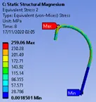 |
1. As the yeild strength of magnesium is less as compared to copper and aluminium, it produces less stress. |
|
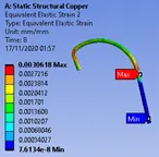
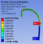
Equivalent elastic strain – Wire |
 |
 |
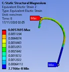 |
1. As the highest young’s modulus of copper it produces less elastic strain. 2. Due to lowest young’s modulus, magnesium produces higher elastic strain. |
- CONCLUSSION
Simulation of wire bending process conducted with Copper Alloy NL, Aluminium Alloy NL and Magnesium Alloy NL. From the analysis it is found that each materials producing different results due to its unique properties.
Wherever precision and strength of the job is required, Copper is suggested as it deforms less as compared to Aluminium and Magnesium
If weight is the constrain, then Magnesium can be selected as it is light in density as compared to copper and magnesium.
As Aluminium Alloy produces good strength in light weight conditions, it’s the best suited material for bending application.