Week 5.1 - Mid term project - Solving the steady and unsteady 2D heat conduction problem
Pre-Conditions:
1. Computational area is to be taken as square shape
2. It is assumed nx=ny; [ no of points on xdirection is equivalent to no of points on y-direction]
3. Boundary conditions are
Top Boundary = 600 K
Bottom Boundary = 900 K
Left Boundary = 400 K
Right Boundary = 800 K
4. The initial assumed temperature is 300 K
There are various methods for solving implicit equations
i) Jacobi
ii) Gauss-Seidel
iii) Successive over relaxation
Solution:
The heat equation is a partial differential equation that describes the distribution of heat evolves over time in a solid medium.
For a function u(x,y,z,t) of three spatial variables (x,y,z) and the time variable t, the heat equation is
`(delu)/(delt)=alpha((del^2u)/(delx^2)+(del^2u)/(dely^2)+(del^2u)/(delz^2))`
where, `alpha` is called the thermal diffusivity of the medium.
This type of heat transfer may occur under two conditions
• Steady state condition
• Unsteady/Transient state condition
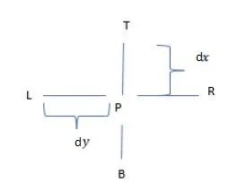
dx- the distance between point T and P
dy- the distance between point L and P
Steady State Equation Discretization
In steady state conduction, the amount of heat entering any region of an object is equal to the amount of heat coming out of it.
`(del^2T)/(delx^2)+(del^2T)/(dely^2)=0`
by discretization this eqation will becomes.
`Tp=1/k[(Tl+Tr)/dx^2+(Tt+Tb)/dy^2]`
Here is the vlue of K
`K=2*((dx^2+dy^2)/(dx^2dy^2))`
Matlab code for steady condition:
clear all
close all
clc;

�fine grid size and boundary conditions
L=1; % length (in m)
H=1; % Height (in m)

nx=10; % Number of nodes in the x-direction
ny=10; % Number of nodes in the y-direction

x=linspace(0,L,nx);
y=linspace(0,H,ny);

dx=L/(nx-1); % dx- the distance between point T and P
dy=H/(ny-1); % dy- the distance between point L and P

T=zeros(nx,ny); % Initial temperature distribution

T(1, :)   = 600;   % Top Boundary
T(end, :) = 900; % Bottom Boundary
T(:, 1)   = 400;   % Left Boundary
T(:, end) = 800; % Right Boundary

T_old=T; %creating a copy of T
omega = 1.1; % Typical values range from 1 to 2 for SOR.

% Convergence criteria
error=9e9;
tol=1e-4;

%User input for selection of methods
method=input("Enter Method--> 1 for Jacobi, 2 for Gauss-seidel and 3 for Successive over-relaxation: ");

if method==1 or Jacobi method
     jacobi_iter=1;

    while error>tol
     for i=2:nx-1
         for j=2:ny-1
            T(i,j)=0.25*(T_old(i-1,j)+T_old(i+1,j)+T_old(i,j-1)+T_old(i,j+1));
         end
     end
     error=abs(max(max(T-T_old)));
     T_old=T;
     jacobi_iter= jacobi_iter+1;

contourf(x,y,T,'ShowText','on')
set(gca,'YDIR','reverse')
xlabel('Length')
ylabel('Height')
title(sprintf('2D heat conduction using Jacobi method in steady state \n Number of iterations:%d',jacobi_iter))
colorbar
colormap(jet)
    end

elseif method==2 /or Gauss-seidel method
    gs_iter=1;

    while error>tol
     for i=2:nx-1
         for j=2:ny-1
             T(i,j)=0.25*(T(i-1,j)+T(i+1,j)+T(i,j-1)+T(i,j+1));
         end
     end
     error=abs(max(max(T-T_old)));
     T_old=T;
     gs_iter= gs_iter+1;
    end

contourf(x,y,T,'ShowText','on')
set(gca,'YDIR','reverse')
xlabel('Length')
ylabel('Height')
title(sprintf('2D heat conduction using Gauss-seidel method in steady state \n Number of iterations:%d',gs_iter))
colorbar
colormap(jet)

elseif method==3  ?or Successive over-relaxation method
    sor_iter=1;
    while error > tol
    for i = 2:nx-1
        for j = 2:ny-1
            new_T = 0.25 * (T(i-1, j) + T(i+1, j) + T(i, j-1) + T(i, j+1));
            T(i, j) = (1 - omega) * T(i, j) + omega * new_T;
        end
    end
    error = max(max(abs(T - T_old)));
    T_old = T;
    sor_iter = sor_iter + 1;
   end

contourf(x, y, T, 'ShowText', 'on')
set(gca, 'YDir', 'reverse')
xlabel('Length')
ylabel('Height')
title(sprintf('2D heat conduction using SOR Method in steady state \n Number of iterations: %d', sor_iter))
colorbar
colormap(jet)
else
    disp('Enter Valid Number')
end
Result:-
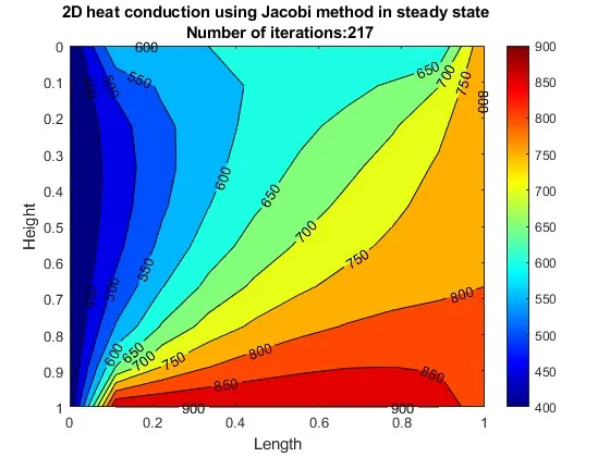
Output of Jacobi Method for Steady State Condition:
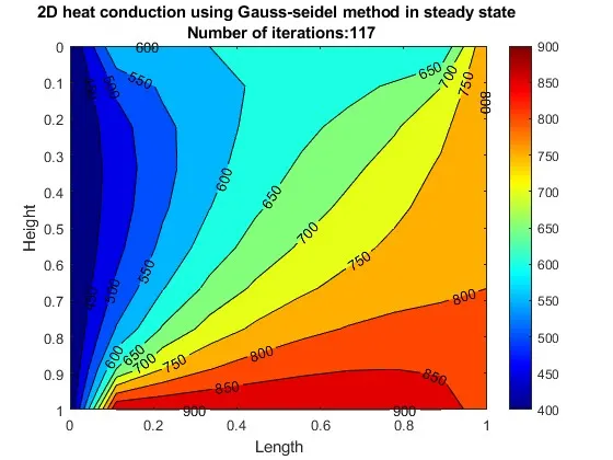
Output of Gauss-Seidel Method for Steady State Condition:
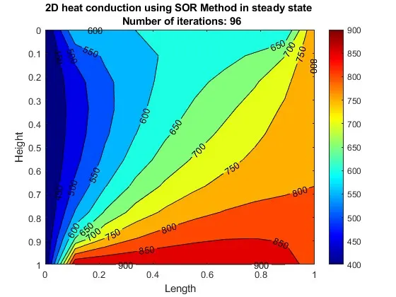
Output of SOR-Sucessive Over-Relaxation method for Steady State Condition:
Observations:
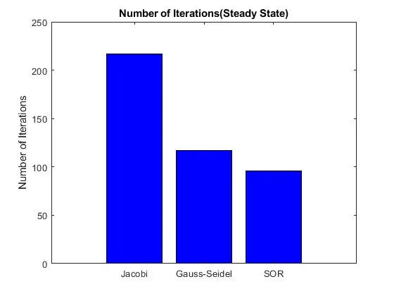
- On comparing the three iterative techniques, it was found that the computational time required to converge the solution was highest in the Jacobi Method as it doesn’t update its values and continues with the guess value.
- Whereas the Gauss-Seidel Method, it uses the updated value of the previous iteration.
- The no of iterations required to converge the solution is less in the SOR Method due to the use of a relaxation factor. If, the omega >1, then it is called over relaxation and the solution get converge faster. If the correction factor is higher than required, then the solution can blow instead of converging and the solution diverges.
- As shown in bar graph, no of iterations varies upon method used.
Implicit Approach Unsteady /Transient -state condition:
Non -steady state:
Non-steady-state situations appear after an imposed change in temperature at a boundary as well as inside of an object, as a result of new source or sink of heat suddenly introduced within an object, causing temperatures near the source or sink to change in time.
`(delT)/(delt)=alpha(del^2T)/(delx^2)+(del^2T)/(dely^2)`
On discretization of Unsteady-State equation :-
`(Tp^(n+1)-Tp^n)/dt=alpha*(Tl-2Tp+Tr)/(delx^2)+(Tt-2Tp+Tb)/(dely^2)`
on further simplyfying it,
`Tp^(n+1)=1/(1+K1+K2)(Tp^n+K1(Tl+Tr)^(n+1)+K2(Tb+Tt)^(n+1))`
where `K1=alpha*dt/dx^2 ,K2=alpha*dt/dy^2`
`alpha`=Thermal diffusity
Explicit Scheme-Unsteady / Transient state:
Condition Unsteady-state Equation discretization (EXPLICIT):
`(delT)/(delt)=alpha*(del^2T)/(delx^2)+(del^2T)/(dely^2)`
we discretize the equation (Explicit)
`(Tp^(n+1)-Tp^n)/dt=alpha*(Tl-2Tp+Tr)/(delx^2)+(Tt-2Tp+Tb)/(dely^2)`
on further simplyfying it,
`Tp^(n+1)=Tp^n+K1(Tl-2Tp+Tb)^n+K2(Tt-2Tp+Tb)^n`
Matlab code for unsteady condtion:
clear all
close all
clc;

�fine grid size and boundary conditions
L=1; % length (in m)
H=1; % Height (in m)

nx=10; % Number of nodes in the x-direction
ny=10; % Number of nodes in the y-direction

x=linspace(0,L,nx);
y=linspace(0,H,ny);


dx=L/(nx-1); % dx- the distance between point T and P
dy=H/(ny-1); % dy- the distance between point L and P

T=300*ones(nx,ny); % Initial temperature distribution

T(1, :)   = 600;   % Top Boundary
T(end, :) = 900; % Bottom Boundary
T(:, 1)   = 400;   % Left Boundary
T(:, end) = 800; % Right Boundary

alpha= 0.01; % approximate thermal diffusivity value
dt=0.1;    �L= (c*dt)/dx
K1=(alpha*dt)/(dx^2);
K2=(alpha*dt)/(dy^2);
K=K1+K2;
timeSteps = 200; % no of time steps
T_old=T; %creating a copy of T
T_prev_dt = T;% copy of T for previous time_step
omega = 1.1; % Typical values range from 1 to 2 for SOR.

% Convergence criteria
error=9e9;
tol=1e-4;

%User input for selection of approach
approach=input("Enter approach--> 1 for implicit, 2 for explicit: ");

if approach==1 %implicit
    %User input for selection of method
    method=input("Enter Method--> 1 for Jacobi, 2 for Gauss-seidel and 3 for Successive over-relaxation: ");
 if method==1 or Jacobi method
     jacobi_iter=1;
  for time_loop=1:timeSteps
    while error > tol
     for i=2:nx-1
         for j=2:ny-1
            term1=((1+(2*K1))+(2*K2))^-1;
                term2=K1*term1;
                term3=K2*term1;
                H=(T_old(i-1,j)+T_old(i+1,j));
                V=(T_old(i,j-1)+T_old(i,j+1));
                T(i,j)=(T_prev_dt(i,j)*term1)+(H*term2)+(V*term3);
         end
     end
     error = max(max(abs(T_old-T)));
     T_old=T;
     jacobi_iter= jacobi_iter+1;
    end
    T_prev_dt=T;
    error=9e9;
 end
contourf(x,y,T,'ShowText','on')
set(gca,'YDIR','reverse')
xlabel('Length')
ylabel('Height')
title(sprintf('2D heat conduction using Jacobi method in Transient state \n Number of iterations:%d',jacobi_iter))
colorbar
colormap(jet)


elseif method==2 /or Gauss-seidel method
    gs_iter=1;
for time_loop=1:timeSteps
 while error > tol
    for i = 2:nx-1
        for j = 2:ny-1
            term1 = (1 + 2 * K1 + 2 * K2)^(-1);
            term2 = K1 * term1;
            term3 = K2 * term1;
            H = T(i-1, j) + T(i+1, j);
            V = T(i, j-1) + T(i, j+1);
            T(i,j)=(T_prev_dt(i,j)*term1)+(H*term2)+(V*term3);
        end
    end
     error = max(max(abs(T_old - T)));
     T_old=T;
     gs_iter= gs_iter+1;
end
T_prev_dt=T;
error=9e9;
end

contourf(x,y,T,'ShowText','on')
set(gca,'YDIR','reverse')
xlabel('Length')
ylabel('Height')
title(sprintf('2D heat conduction using Gauss-seidel method in Transient state \n Number of iterations:%d',gs_iter))
colorbar
colormap(jet)


elseif method==3  ?or Successive over-relaxation method
    sor_iter=1;
 for time_loop=1:timeSteps
    while error > tol
    for i = 2:nx-1
        for j = 2:ny-1
            term1 = (1 + 2 * K1 + 2 * K2)^(-1);
            term2 = K1 * term1;
            term3 = K2 * term1;
            H = T(i-1, j) + T(i+1, j);
            V = T(i, j-1) + T(i, j+1);
            new_T=(T_prev_dt(i,j)*term1)+(H*term2)+(V*term3);
            T(i, j) = (1 - omega) * T(i, j) + omega * new_T;
        end
    end
    error = max(max(abs(T - T_old)));
    T_old = T;
    sor_iter = sor_iter + 1;
   end
T_prev_dt=T;
error=9e9;
end
contourf(x, y, T, 'ShowText', 'on')
set(gca, 'YDir', 'reverse')
xlabel('Length')
ylabel('Height')
title(sprintf('2D heat conduction using SOR Method in Transient state \n Number of iterations: %d', sor_iter))
colorbar
colormap(jet)
else
    disp('Enter Valid Number')
end

% Explicit approach

elseif approach==2
  for time_loop=1:timeSteps
     for i=2:nx-1
         for j=2:ny-1
                H=(T_old(i-1,j)-2*T_old(i,j)+T_old(i+1,j));
                V=(T_old(i,j-1)-2*T_old(i,j)+T_old(i,j+1));
                T(i,j)=T_old(i,j)+(K1*H)+(K2*V);
         end
     end
     T_old=T;
  end
contourf(x,y,T,'ShowText','on')
set(gca,'YDIR','reverse')
xlabel('Length')
ylabel('Height')
title(sprintf('2D heat conduction using in Transient state by Explicit approach'))
colorbar
colormap(jet)

    else
        disp('Valid approach');
end
Result:-
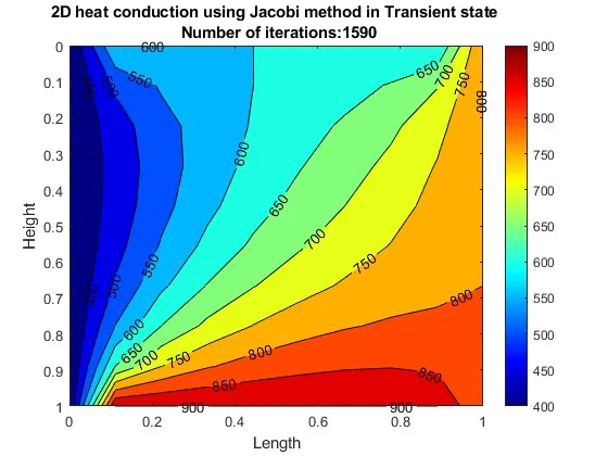
Output of Jacobi Method in Transient State using Implicit approach:
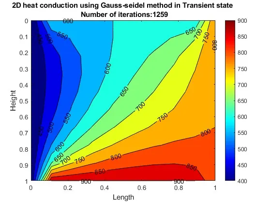
Output of Gauss-Seidel Method in Transient State using Implicit approach:
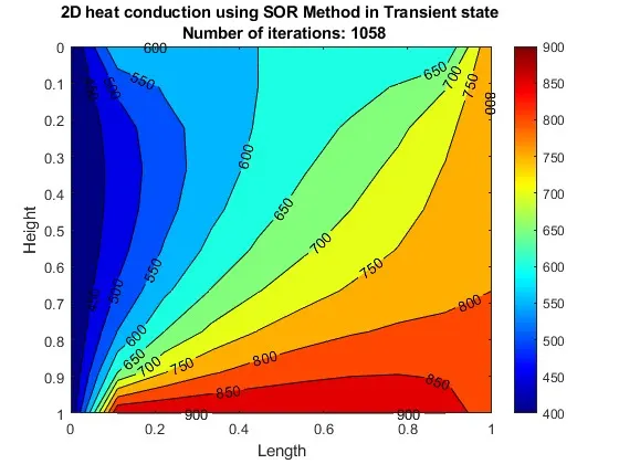
Output of SOR-Sucessive Over-Relaxation method in Transient State using Implicit approach:
Observations:
- The transient analysis gives better performance compared to the steady-state as it depicts the realworld scenario.
- The transient analysis takes into consideration the varying rate of heat transfer with respect to time.
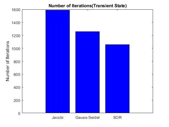
- Similar to steady-state analysis, the no of iterations required to converge the solution was falling from the Jacobi method to the SOR Method as depicted by the bar graph.
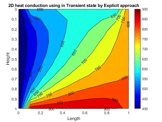
Result of Explicit approach- Transient condition:
Observations:
- The graph represents the temperature distribution at a specific time step during the simulation. As the simulation progresses, the temperature distribution evolves over time.
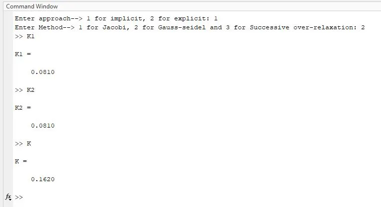
- According to CFL stability criteria, K1+K2 i.e. K <0>