Week 5 - Curve fitting
popt: It stands for "optimal parameters." When using curve_fit, popt contains the values of the parameters that minimize the difference between the fitted function and the data. For example, if you're fitting a linear equation y=mx+b, popt will contain the values of m (slope) and b (intercept).
pcov: This stands for "covariance of the parameters." It is a matrix that provides an estimate of the uncertainties (standard deviations) of the parameters inpopt. The diagonal elements of this matrix give the variance of the fitted parameters. The square root of the diagonal elements gives the standard deviation (errors) of the parameters.
2)np.array(temperature) converts the list temperature (or another sequence like tuples or lists) into a NumPy array. NumPy arrays are useful because they allow for vectorized operations, meaning you can perform mathematical operations on entire arrays efficiently.
temperature = [100, 200, 300, 400]3.) What does the * in *popt mean?
The * in *popt is used for unpacking the elements in popt. Suppose popt contains two values, like the slope and intercept of a linear fit, using *popt allows you to pass those two values separately as arguments
def linear_func(x, a, b):
return a * x + b
popt = [2, 3] # a=2, b=3
result = linear_func(x, *popt) # equivalent to linear_func(x, 2, 3)
4)4. Write code to fit a linear and cubic polynomial for the Cp data. Explain if your results are good or bad.
program:-
import numpy as np
import matplotlib.pyplot as plt
from scipy.optimize import curve_fit
# Example Cp data
temperature = np.array([100, 200, 300, 400, 500, 600])
Cp = np.array([1.2, 1.8, 3.4, 5.6, 7.3, 9.1])
# Define the linear and cubic models
def linear_func(T, a, b):
return a * T + b
def cubic_func(T, a, b, c, d):
return a * T**3 + b * T**2 + c * T + d
# Fit the linear model
popt_linear, pcov_linear = curve_fit(linear_func, temperature, Cp)
# Fit the cubic model
popt_cubic, pcov_cubic = curve_fit(cubic_func, temperature, Cp)
# Generate data for plotting the fit
T_fit = np.linspace(min(temperature), max(temperature), 100)
Cp_linear_fit = linear_func(T_fit, *popt_linear)
Cp_cubic_fit = cubic_func(T_fit, *popt_cubic)
# Plot the data and fits
plt.scatter(temperature, Cp, label='Data')
plt.plot(T_fit, Cp_linear_fit, label='Linear Fit', color='red')
plt.plot(T_fit, Cp_cubic_fit, label='Cubic Fit', color='green')
plt.xlabel('Temperature')
plt.ylabel('Cp')
plt.legend()
plt.show()
# Print the fitted parameters
print(f'Linear Fit Parameters: {popt_linear}')
print(f'Cubic Fit Parameters: {popt_cubic}')
import numpy as np
import matplotlib.pyplot as plt
from scipy.optimize import curve_fit
# Example Cp data
temperature = np.array([100, 200, 300, 400, 500, 600])
Cp = np.array([1.2, 1.8, 3.4, 5.6, 7.3, 9.1])
# Define the linear and cubic models
def linear_func(T, a, b):
return a * T + b
def cubic_func(T, a, b, c, d):
return a * T**3 + b * T**2 + c * T + d
# Fit the linear model
popt_linear, pcov_linear = curve_fit(linear_func, temperature, Cp)
# Fit the cubic model
popt_cubic, pcov_cubic = curve_fit(cubic_func, temperature, Cp)
# Generate data for plotting the fit
T_fit = np.linspace(min(temperature), max(temperature), 100)
Cp_linear_fit = linear_func(T_fit, *popt_linear)
Cp_cubic_fit = cubic_func(T_fit, *popt_cubic)
# Plot the data and fits
plt.scatter(temperature, Cp, label='Data')
plt.plot(T_fit, Cp_linear_fit, label='Linear Fit', color='red')
plt.plot(T_fit, Cp_cubic_fit, label='Cubic Fit', color='green')
plt.xlabel('Temperature')
plt.ylabel('Cp')
plt.legend()
plt.show()
# Print the fitted parameters
print(f'Linear Fit Parameters: {popt_linear}')
print(f'Cubic Fit Parameters: {popt_cubic}')
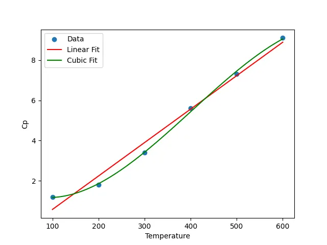
Results:-
Linear fit: If the Cp data is more complex (e.g., curving or nonlinear), the linear model may not fit well. You might see that the red line doesn't capture the trend of the data points
Cubic fit: A cubic model is more flexible and may provide a better fit, especially if the data shows nonlinearity. However, be cautious—overfitting can happen if the model is too complex, especially with limited data points.
5) What needs to be done in order to make the curve fit perfect?
ans:-Increase the complexity of the model: If the data shows a non-linear trend, use a higher-degree polynomial or a more complex model that captures the non-linearity.
Increase data points: More data points improve the fit because they reduce the chance of overfitting and provide more information for the model.
Regularization: To avoid overfitting with higher-order polynomials, techniques like L2 regularization can help.
Use non-linear fitting functions: If polynomials don't work, use other functions such as logarithmic, exponential, or even a combination of functions depending on the dataset's behavior
6) ans:-
A few methods can be used to assess how well the model fits the data:
R-squared: This statistic explains the proportion of variance in the dependent variable that the model captures.
Residuals: Plot the residuals (differences between the actual data and the fitted curve). Ideally, residuals should be randomly distributed with no clear pattern
Chi-squared or RMSE (Root Mean Square Error): These are metrics that quantify the error between the observed and predicted data.