Week 5 - Rayleigh Taylor Instability

Rayleigh-Taylor instability (RTI) is the interpenetration of materials that occurs whenever a light fluid pushes on a heavy fluid. It is a dynamic process whereby the two fluids seek to reduce their combined potential energy. The ensuing turbulence and mixing has far-reaching consequences in many natural and man-made flows, ranging from supernovae to inertial confinement fusion (ICF) capsules.

Euler-Lagrange approach

The Lagrangian discrete phase model follows the Euler-Lagrange approach. The fluid phase is treated as a continuum by solving the Navier-Stokes equations, while the dispersed phase is solved by tracking a large number of particles, bubbles, or droplets through the calculated flow field. The dispersed phase can exchange momentum, mass, and energy with the fluid phase.

Euler-Euler Approach

In Fluent three different Euler-Euler multiphase models are available:        

• Volume of fluid (VOF) model
• Mixture model 
• Eulerian model

The VOF Model

The VOF model  is a surface-tracking technique applied to a fixed Eulerian mesh. It is designed for two or more immiscible fluids where the position of the interface between the fluids is of interest.

The Mixture Model

The mixture model is designed for two or more phases (fluid or particulate). As in the Eulerian model, the phases are treated as interpenetrating continua. 

The Eulerian Model

The Eulerian model is the most complex of the multiphase models in. It solves a set of momentum and continuity equations for each phase. 

Aim :-

Create The Geometry 2D

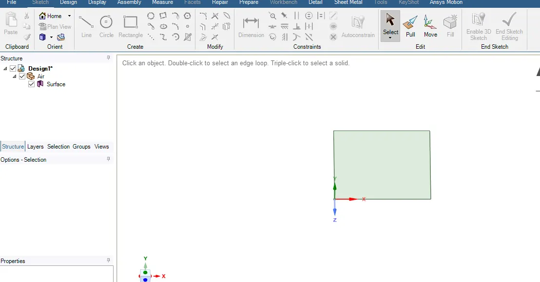
Ansys Workbench→Ansys Fluent →Geometry (Open With New Speci claim) →Design →Rectangle 20x20→use pull tool for create surface.→In Tree Change the component surface as a component.

Create another New Component →Water →Sketch the rectangle 20x20→and pull surface

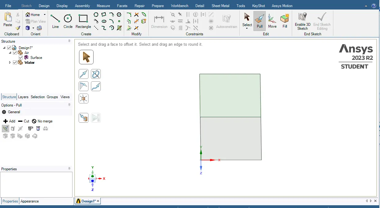
For confirmational mesh we use to join two surface then we can follow the steps 2 D geometry.

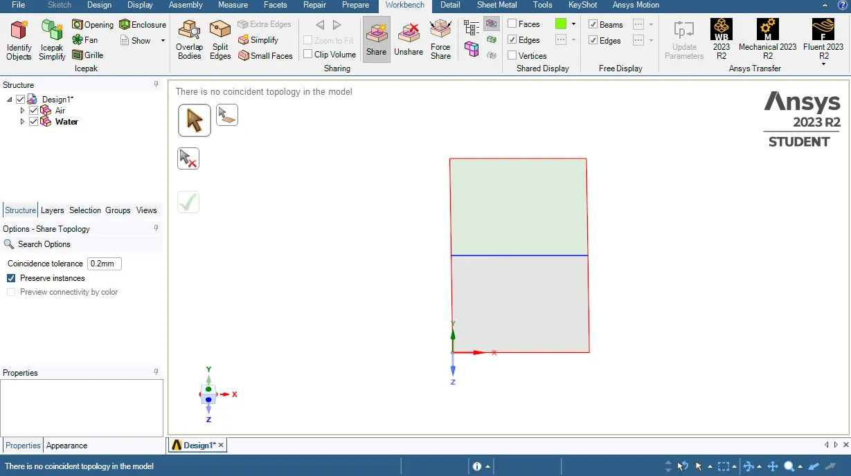
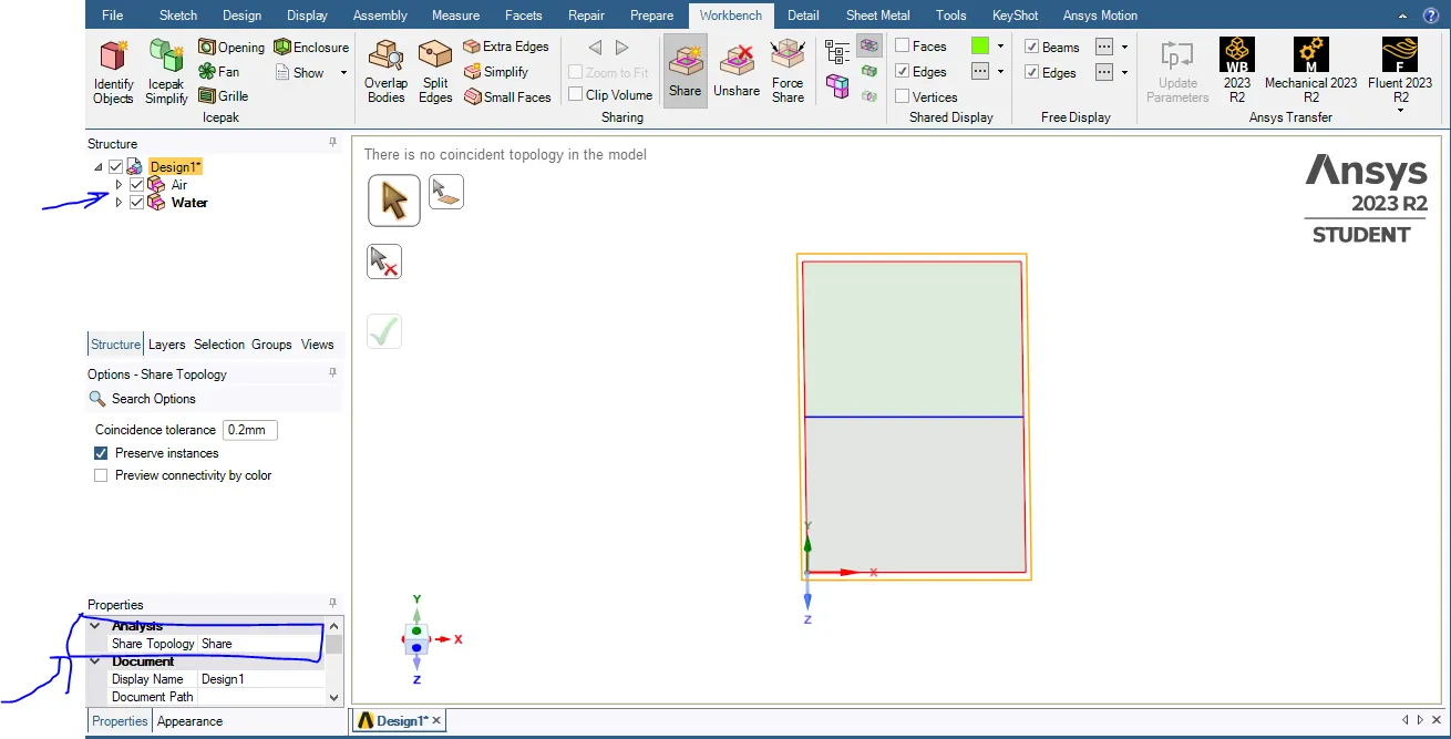
Geometry→Workbench→Select the both Geometry→click on share→Ok→ after that one window information shows that 1 edge is shared → we can see on tree model is changes and topology is shared.

Meshing

Genrate the Basic Mesh.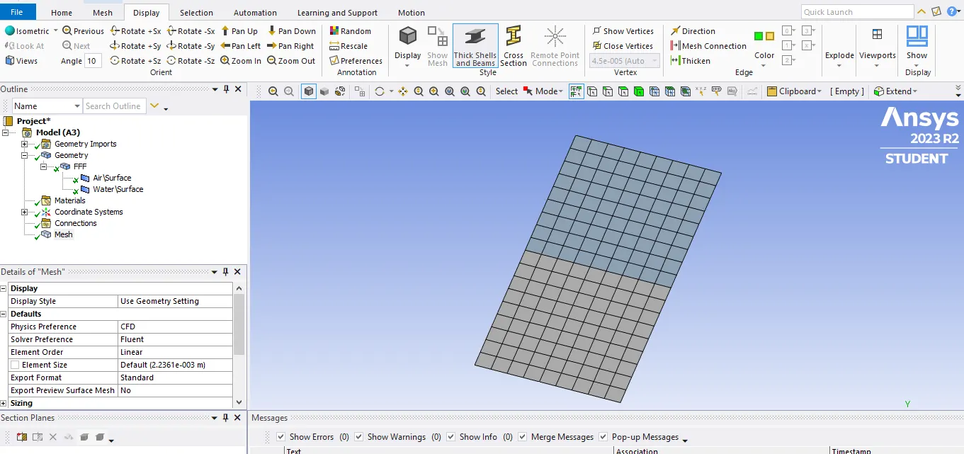

Genrate the Basic Mesh.0.5mm

Setup :-

Domain 

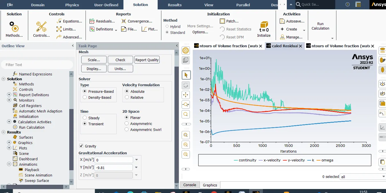
Transient

Gravity- y -9.8 m/s⊃2;

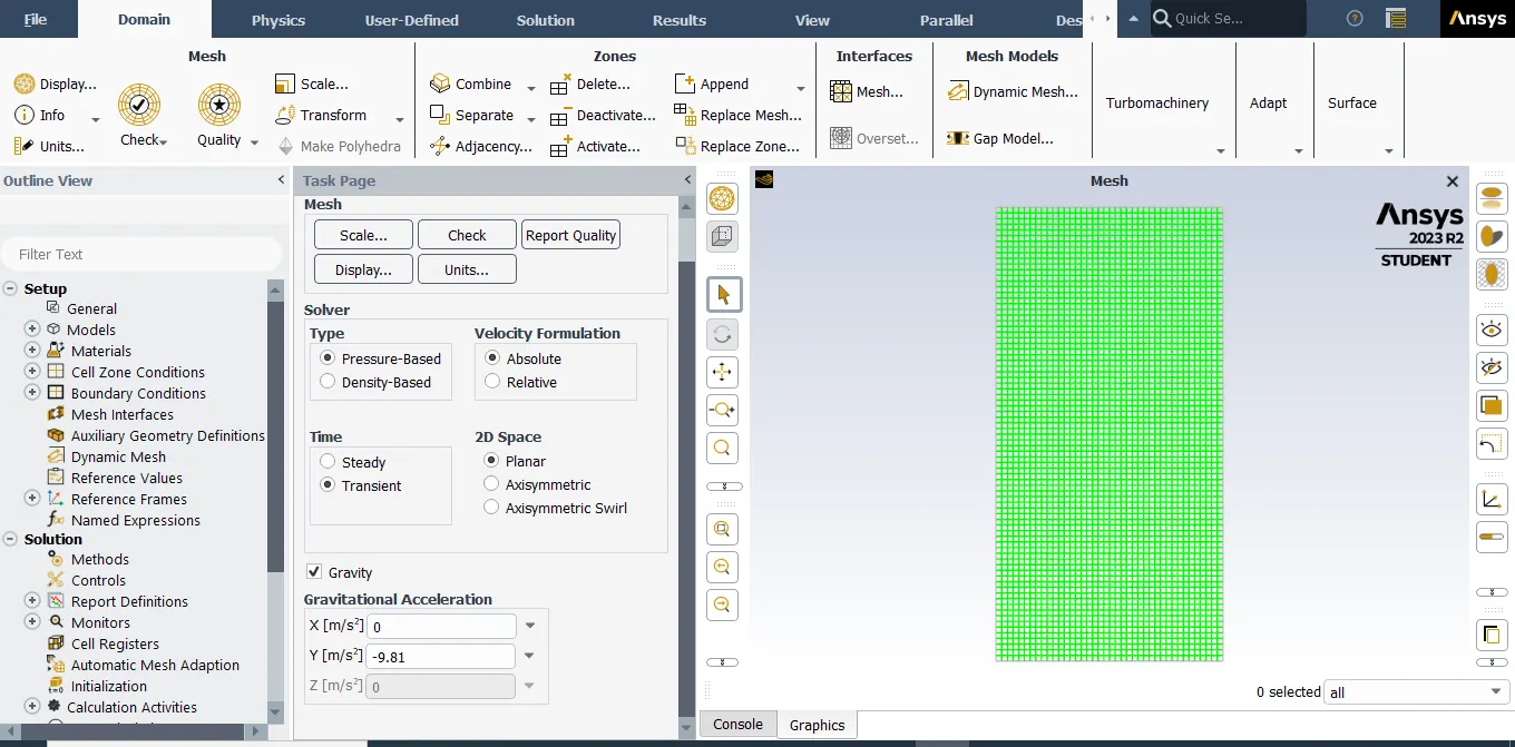
Setup Physics

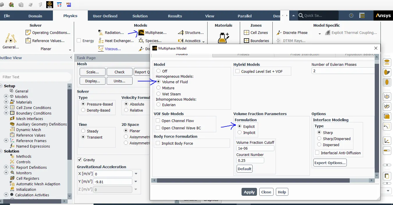
Multi Phase Model→Volume of fluid→explicit Method→ok

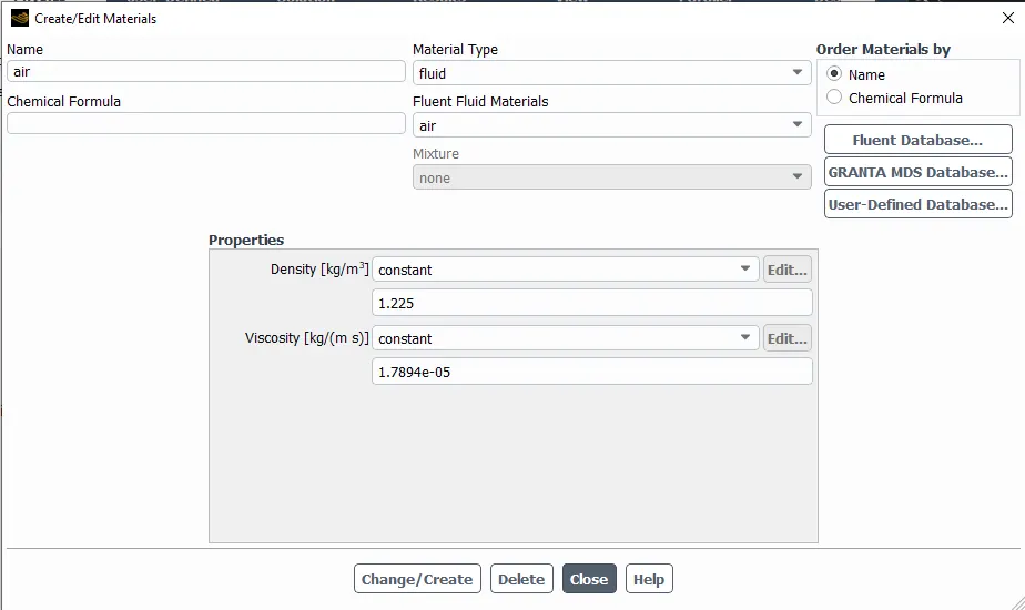
Material:-

Air & Water (L)

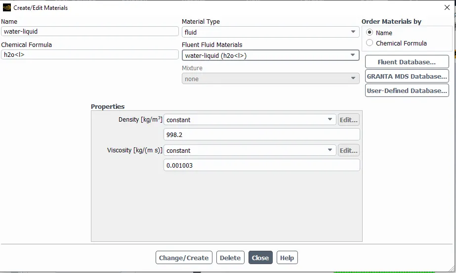
Select the phases

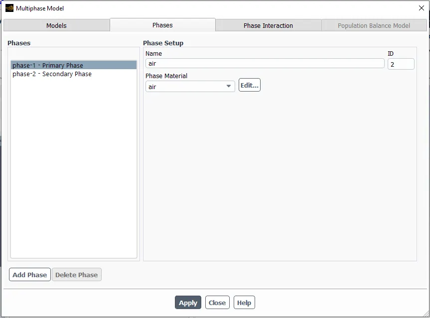
Multiphase → select Phase setup → select the primary Phase → Insert Name air → select material Air

 

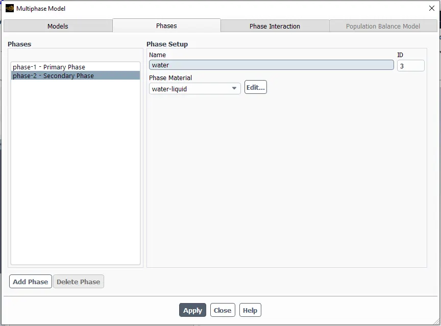
Multiphase → select Phase setup → select the Secondary Phase → Insert Name Water → select material Water.

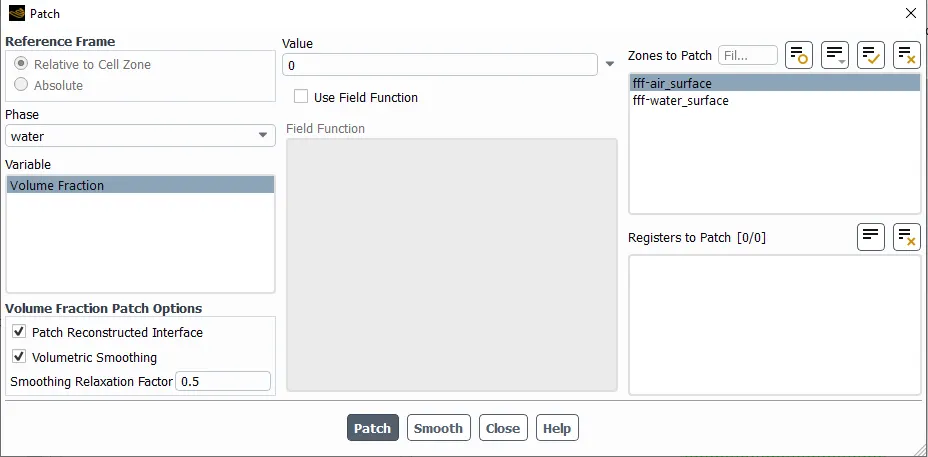
iteration is not performed that we setup the patching process for setup intialization.

Solution→Intialization→Phase(water)→Selcet Zone-Air & Water →value for air is 0 & Water 1 →patch it

Creates the contour

Result→Contour →new →select phase → All Phases display →ok

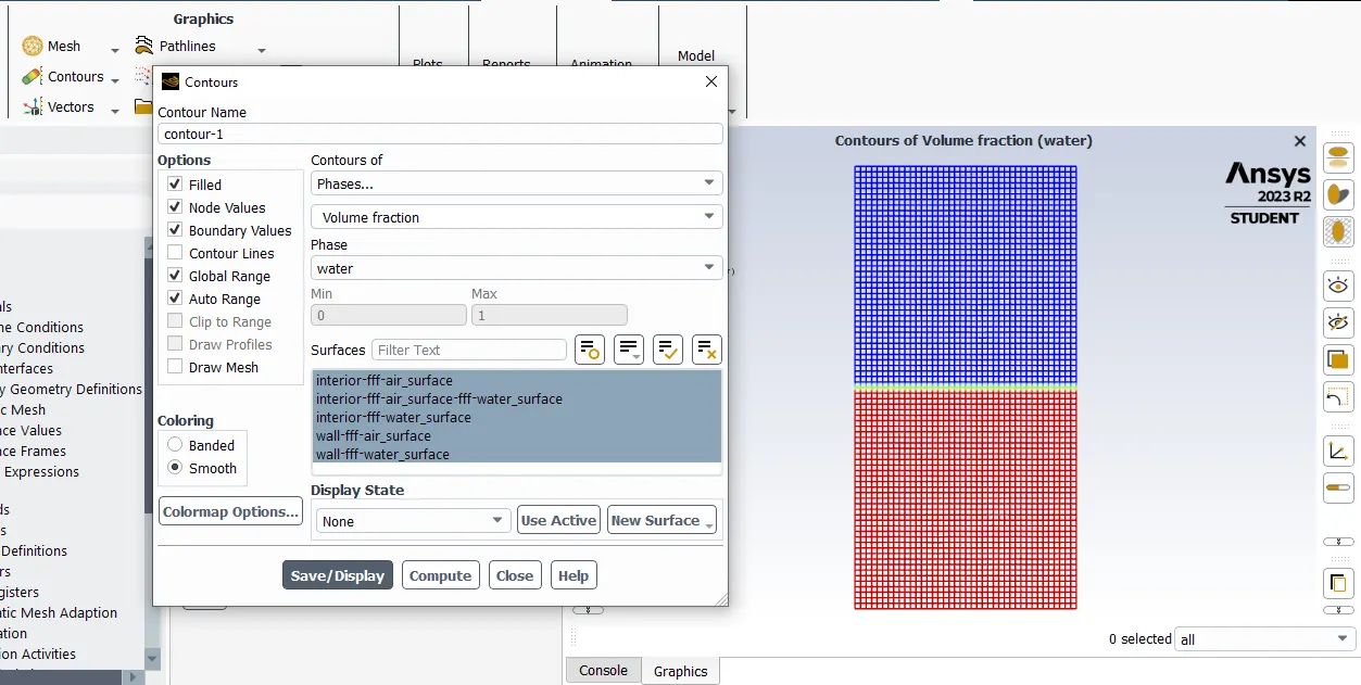
Create Animation

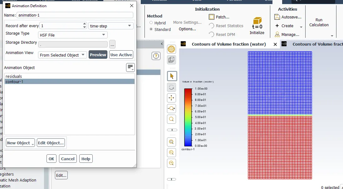
itration & Time

result

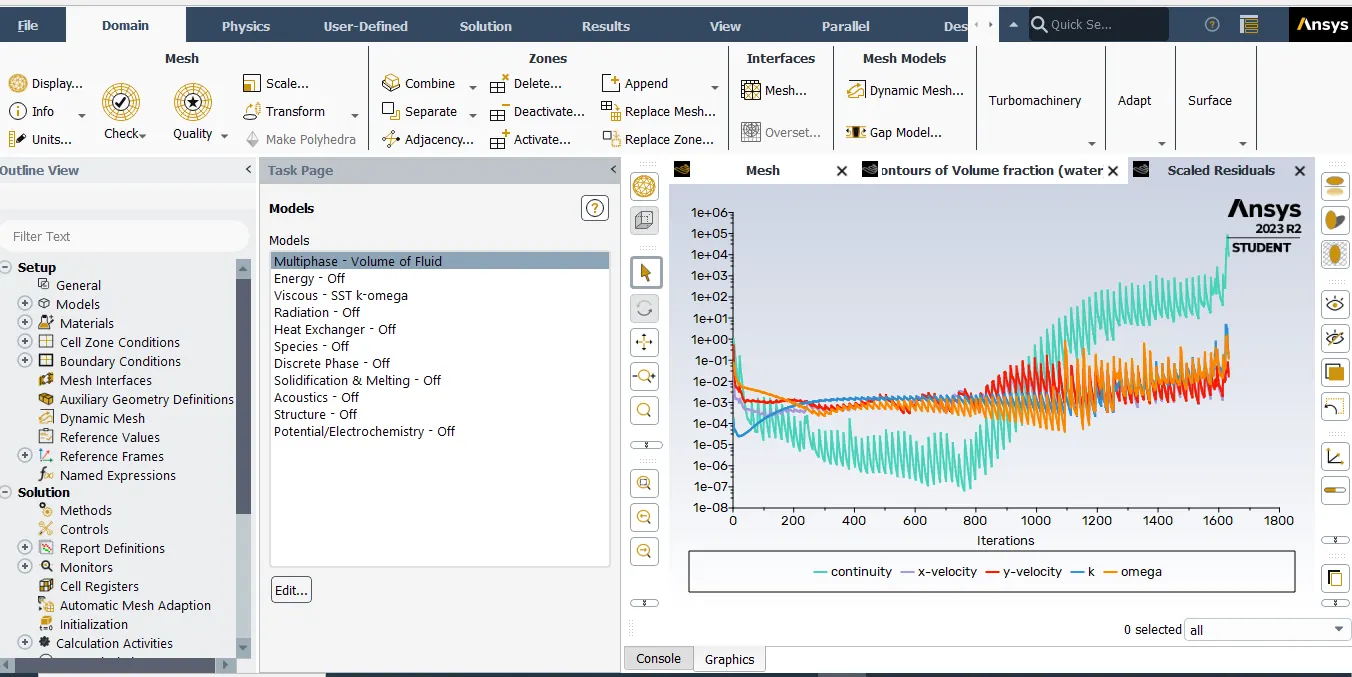
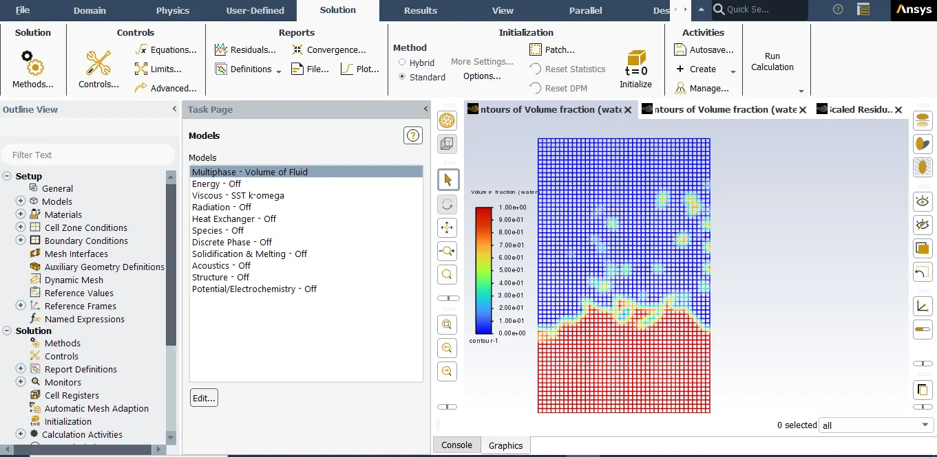
Animation Video Link:-

https://drive.google.com/file/d/1H4lkiyXuAFmVOjQM0PiQUPLOlFuhAyUT/view?usp=sharing

Case -2 Genrate the Basic Mesh.0.1 mm

Setup :-

Domain 

Transient

Gravity- y -9.8 m/s⊃2;

 

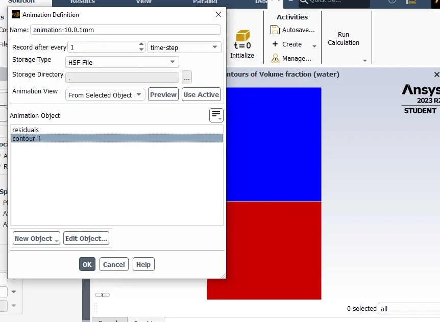
Animation Video Link:

 https://drive.google.com/file/d/1Kfn8eIeeHcjvkKWjMTG76volUeOAnM5q/view?usp=sharing

Define the Atwood Number. Find out the Atwood number for both the cases and explain how the variation in Atwood number in the above two cases affects the behavior of the instability.

Define Atwood Number

The Atwood number (A) is a dimensionless number in fluid dynamics used in the study of hydrodynamic instabilities in density stratified flows. It is a dimensionless density ratio defined as:

`A = (rho_1 - rho_2)/(rho_1+rho_2)`

Where, `rho_1` - density of Heavier Fluid

           `rho_2` - density of lighter fluid

 CONCLUSION

• From the above cases, we observe that finer mesh captures the instability better than the coarse mesh, but it takes more time for the heavier fluid to settle down. As computational time is long but produces results with better accuracy.
• Since the simulation involves capturing instabilities that are changing in an unpredictable manner as a function of time, the transient approach is preferred over the steady-state approach. 

• For Atwood number close to 0, RT instability flows take the form of symmetric fingers of fluid.
• when Atwood number close to 1, the much lighter fluid below the heavier fluid takes the form of larger bubble-like plumes.