Week 3 - Solving second order ODEs

Ans :- step wise explanation of the code

. numpy (np): Used for numerical operations and array handling.

matplotlib.pyplot (plt): For plotting and visualizing the pendulum's motion.

scipy.integrate.solve_ivp: To solve the system of ordinary differential equations (ODEs).

matplotlib.animation.FuncAnimation: To animate the pendulum’s motion.

Defining parameters:-These parameters represent the physical properties of the pendulum, such as gravity, length, mass, and damping coefficient.

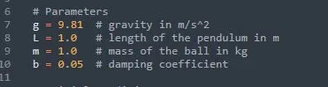
Initial Conditions and Time Span

• $\frac{d\theta}{dt} = \omega$
  
• $\frac{d\omega}{dt} = -\frac{b}{m} \omega - \frac{g}{L} \sin(\theta)$
  
• 
  
• 
  
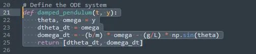
• solving the ode.
  
• 
  
• exacting the solution
  
• The solution contains arrays for angular displacement (theta), angular velocity (omega), and the corresponding time points (time)
  
• 
  
• Converting Angle to Cartesian Coordinates
  
• 
  
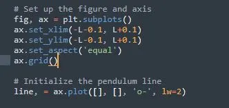
• setup the plots
  
• 
  
• 
  
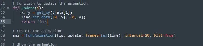
• define animation code
  
• 
  
• display.
  
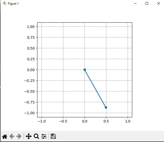
• graph and animation.
  
• 
  
• error faced in the program.
• sealing mistake in the import code.
• 
  
• in this library i have extra s added then, i removed the function library is correct shows
  
• have not defined the function equation did not wrote
• equation write then code is exicute.
• Approach: Re-examined the function snimstion setup, particularly the update function and how the pendulum’s coordinates were updated.
  
• resolution: Ensured that the update function correctly accessed the time-indexed values of theta and properly updated the line's
  
• conclusion:- pendulum second order equation is running simulation as per given problem smoothly.

Code :-

import numpy as np

import matplotlib.pyplot as plt

from scipy.integrate import solve_ivp

from matplotlib.animation import FuncAnimation

# Parameters

g = 9.81 # gravity in m/s^2

L = 1.0 # length of the pendulum in m

m = 1.0 # mass of the ball in kg

b = 0.05 # damping coefficient

# Initial conditions

theta0 = 0.0 # initial angular displacement in radians

omega0 = 3.0 # initial angular velocity in rad/s

# Time span

t_span = (0, 20) # simulate between 0 and 20 seconds

t_eval = np.linspace(t_span[0], t_span[1], 1000) # 1000 time points for evaluation

# Define the ODE system

def damped_pendulum(t, y):

theta, omega = y

dtheta_dt = omega

domega_dt = -(b/m) * omega - (g/L) * np.sin(theta)

return [dtheta_dt, domega_dt]

# Solve the ODE

sol = solve_ivp(damped_pendulum, t_span, [theta0, omega0], t_eval=t_eval)

# Extract the solution

theta = sol.y[0]

omega = sol.y[1]

time = sol.t

# Function to convert angle to x, y coordinates for plotting

def get_xy(theta):

x = L * np.sin(theta)

y = -L * np.cos(theta)

return x, y

# Set up the figure and axis

fig, ax = plt.subplots()

ax.set_xlim(-L-0.1, L+0.1)

ax.set_ylim(-L-0.1, L+0.1)

ax.set_aspect('equal')

ax.grid()

# Initialize the pendulum line

line, = ax.plot([], [], 'o-', lw=2)

# Function to update the animation

def update(i):

x, y = get_xy(theta[i])

line.set_data([0, x], [0, y])

return line,

# Create the animation

ani = FuncAnimation(fig, update, frames=len(time), interval=20, blit=True)

# Show the animation

plt.show()

video link :- https://www.youtube.com/watch?v=GQBdZ9-SWX0