Week 4.1 - Genetic Algorithm

Aim: Write a code in MATLAB to create the stalagmite function

function [f] = stalagmite(input_vector)
x = input_vector(1);
y = input_vector(2);
    f1 = (sin(5.1*pi*x+0.5)).^6;
    f2 = exp((-4*log(2)*((x-0.0667).^2))/0.64);
    f3 = (sin(5.1*pi*y+0.5)).^6;
    f4 = exp((-4*log(2))*((y-0.0667).^2)/0.64);
    
    f = -(f1*f2*f3*f4);
end

Aim : Write a code in MATLAB to optimise the stalagmite function and find the global maxima of the function.

clear all
close all
clc

%stalagmite with Genatic Algorithm
x = linspace(0,0.6,150);
y = linspace(0,0.6,150);

%Meshing
[xx,yy] = meshgrid(x,y);

%looping Stalagmite
for i=1:length(xx)
    for j=1:length(yy)
        input_vector(1)=xx(i,j);
        input_vector(2)=yy(i,j);
        f(i,j)= stalagmite(input_vector);
    end
end

f=-f;
surfc(x,y,f)

shading interp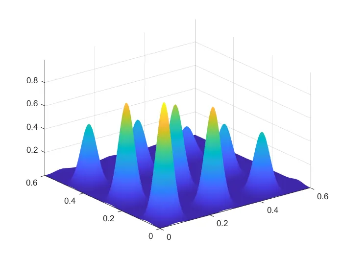

Genetic Algorithm:

Charles Darwin’s theory of natural evolution. A natural selection process where the best value is taken for reproduction to the next generation. This method is used for solving both constrained and unconstrained optimization problems. In simple words, they find “survival of the fittest” among individual of consecutive generation for solving a problem.

****SYNTAX FOR GA IS EXPLAINED IN CODING EXPLANATION PART****

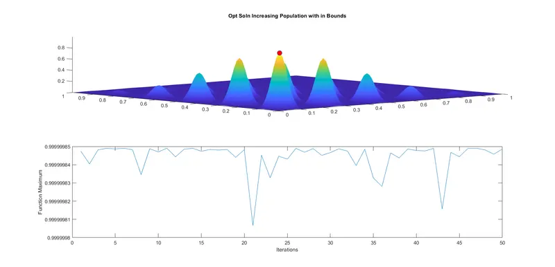
Aim : Plot graphs for all 3 studies and for F maximum vs no. of iterations.

clear all
close all
clc

%Creating search space
x = linspace(0,1,150);
y = linspace(0,1,150);
num_cases = 50

%Meshig Array
[xx yy] = meshgrid(x,y);
 
%looping Stalagmite
for i=1:length(xx)
    for j=1:length(yy)
        input_vector(1)=xx(i,j);
        input_vector(2)=yy(i,j);
        f(i,j)= stalagmite(input_vector);
    end
end

% Study 1 :Programm For unbounded 
tic
for i =1:num_cases
    [Inputs,f_opt(i)] = ga(@stalagmite,2);
    x_opt(i) = Inputs(1);
    y_opt(i) = Inputs(2);
end
study_time1 = toc

figure(1)
subplot(2,1,1)
hold on 

f_opt=-f_opt;
surfc(x,y,-f)
shading interp

plot3(x_opt,y_opt,f_opt,'marker','O','markersize',3,'markerfacecolor','r')
title('Opt Soln Unbounded')
subplot(2,1,2)
plot(f_opt)
xlabel('Iterations')
ylabel('Function Maximum')


% Study 2 :Programm For with Lower & Upper Bounds
tic
for i =1:num_cases
    [Inputs,f_opt(i)] = ga(@stalagmite,2,[],[],[],[],[0;0],[1;1]);
    x_opt(i) = Inputs(1);
    y_opt(i) = Inputs(2);
end
study_time2 = toc

figure(2)
subplot(2,1,1)
hold on 
f_opt=-f_opt;
surfc(x,y,-f)
shading interp

plot3(x_opt,y_opt,f_opt,'marker','O','markersize',3,'markerfacecolor','r')
title('Opt Soln With with Lower & Upper Bounds')
subplot(2,1,2)
plot(f_opt)
xlabel('Iterations')
ylabel('Function Maximum')


% Study 3 :Programm For with Lower & Upper Bounds and increasing population
% size
options = optimoptions('ga');
options = optimoptions(options,'Populationsize',500);

tic
for i =1:num_cases
    [Inputs,f_opt(i)] = ga(@stalagmite,2,[],[],[],[],[0;0],[1;1],[],[],options);
    x_opt(i) = Inputs(1);
    y_opt(i) = Inputs(2);
end
study_time3 = toc

figure(3)
subplot(2,1,1)
hold on 
f_opt=-f_opt;
surfc(x,y,-f)
shading interp

plot3(x_opt,y_opt,f_opt,'marker','O','markersize',10,'markerfacecolor','r')
title('Opt Soln Increasing Population with in Bounds')
subplot(2,1,2)
plot(f_opt)
xlabel('Iterations')
ylabel('Function Maximum')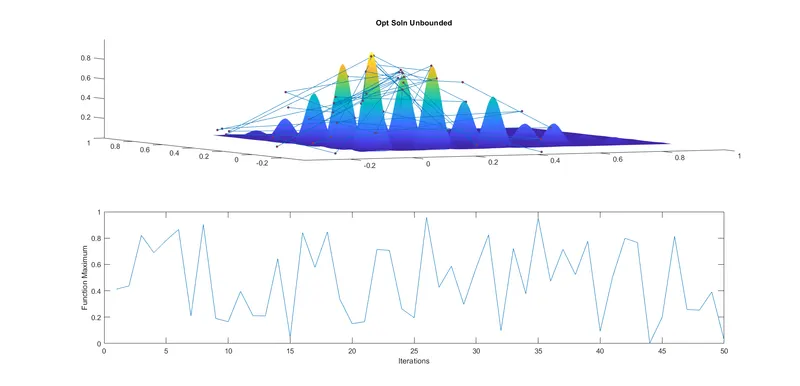

Coding Explanation:

1. Initially X & Y array is defined using linspace at equal intervals.
2. 2D array is created using mesghgrid cmd.
3. iterations is defined as 50
4. Stalagmite function is derived with the formula for stalagmite.
5. input vector is defined and this function is looped in.
6. Then plot is created with stalagmite plot and iteration VS maximum function plot, and this plot is defined in same figure plot.
7. After this a case study is made to get the highest and opted value of stalagmite function using GENETIC ALGORITHM.
8. As the genetic algorithm finds out the least value of the problem, thus the stalagmite funtion is coded with coding concept of GA to find Global Maximum Value.
9. Study Comprises of 3 type
   1. unbounded Inputs
   2. Bounded Inputs
   3. Increased Population with Bounded Inputs
10. In first case the inputs for the variable is set with no limits,no bounds, and no restrictions, with cmd of study time tic-tok to get the duration of the loop takes to cpmplete.Syntax for this GA is x = ga(fun,nvars)
    • fun = objective function(stalagmite)
    • nvars = no.of vaariables(x,y)
      • the values and plot created for this function will be more and the lowest point will be more.
      • So to get more clearer and best value, the GA syntax need to be upgraded.
11. In Second Case the same funtion is upgraded to GA syntax with more specific details like bounding limits, to get even more exact value. Syntax for this GA is x= ga(fun,nvars,A,B,Aeq,Beq,lb,ub)
    • A,B = Linear inequality constraints
    • Aeq,Beq = Linear equality constraints
    • lb = lower bound
    • ub = upper bound
      • Here the data need to filled otherwise pattern search uses the default option values.
      • Linear inequality constraints & Linear equality constraints are not provided, therefore the value for that data is coded as '[]',if not the solver will automaticaly assign value to it.
      • After this function is performed,we can get the values nearer to the exact value.
      • So to get more clearer and best value, the GA syntax is even more upgraded.
12. In Third Case the same funtion is upgraded to GA syntax with more specific details like bounding limits and incrementaion of population,to get even more exact value.The population is increased manually to higher limit, as while looping the loop will go around the bounded limits with maximum population,this will lead to exact least value.
13. There we get the global maxima value. Syntax for this GA is x=ga(fun,nvars,A,b,Aeq,beq,lb,ub,nonlcon,IntCon,options)
    • nonlcon = nonlinear constraints
    • intcon = integer values
    • options = optimization options
      • nonlinear constraints & integer values are not available therefore the value for that data is coded as '[]',if not the solver will automaticaly assign value to it.
      • This will give the exact value we needed, as the looping done inside the population that we increased manually.

Conclusion: Thus the problem is optimized with concept of Genetic Algorithm.