Week 5 - Curve fitting
1.popt and pcov
- Popt-It is an array.This will be our coefficients in the program. It represents the unknowns in the function defined in the program so later it will be the output as it curve fit function calculates it. In other words optimal values for the parameters so that the sum of the squared error is minimized.
- pcov-The estimated covariance of popt. The diagonals provide the variance of the parameter estimate.
2.np.array(temperature)
- np.array(temperature) stores the values of temperature in the form of array and passes it to numpy function.
3.* in *popt
- It stores the values of unknown variables in popt array.
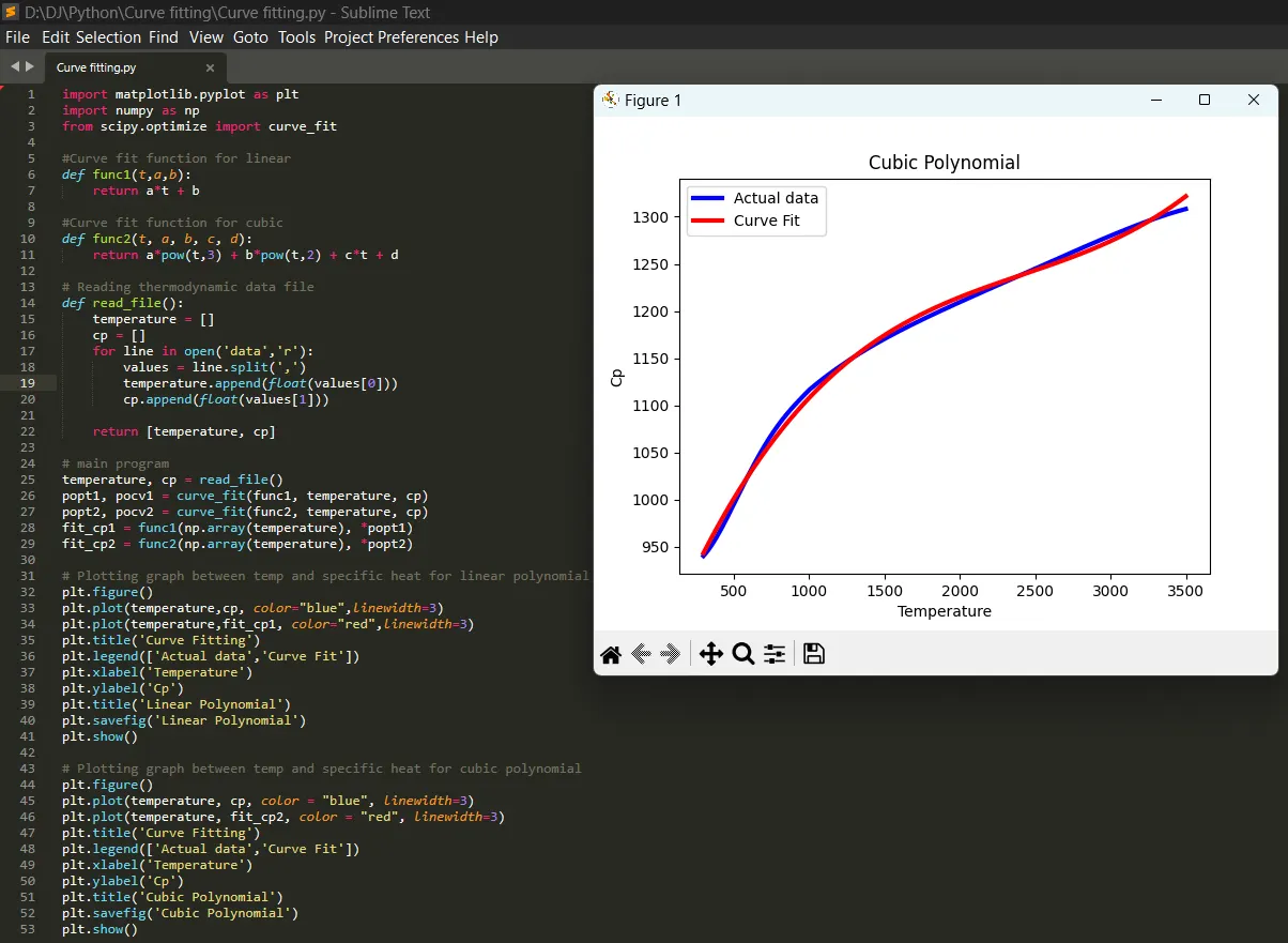
5.The degree of the equation of the curve is directly proportional the level of curve fit accuracy. As the number of coefficients increases the value estimated tend to follow the original curve.
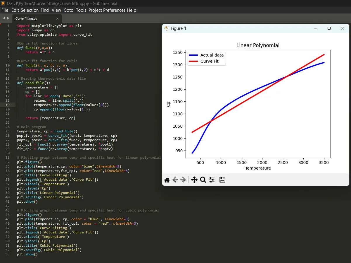
6.AS per the above output, we can see that as the degree of the equation the linear curve fit plot looks a lot different to the original plot. In the quintic fit we can clearly see that the curves overlap signify well performed.
4. Coding:
import matplotlib.pyplot as plt
import numpy as np
from scipy.optimize import curve_fit
#Curve fit function for linear
def func1(t,a,b):
return a*t + b
#Curve fit function for cubic
def func2(t, a, b, c, d):
return a*pow(t,3) + b*pow(t,2) + c*t + d
# Reading thermodynamic data file
def read_file():
temperature = []
cp = []
for line in open('data','r'):
values = line.split(',')
temperature.append(float(values[0]))
cp.append(float(values[1]))
return [temperature, cp]
# main program
temperature, cp = read_file()
popt1, pocv1 = curve_fit(func1, temperature, cp)
popt2, pocv2 = curve_fit(func2, temperature, cp)
fit_cp1 = func1(np.array(temperature), *popt1)
fit_cp2 = func2(np.array(temperature), *popt2)
# Plotting graph between temp and specific heat for linear polynomial
plt.figure()
plt.plot(temperature,cp,,linewidth=3)
plt.plot(temperature,fit_cp1,,linewidth=3)
plt.title('Curve Fitting')
plt.legend(['Actual data','Curve Fit'])
plt.xlabel('Temperature')
plt.ylabel('Cp')
plt.title('Linear Polynomial')
plt.savefig('Linear Polynomial')
plt.show()
# Plotting graph between temp and specific heat for cubic polynomial
plt.figure()
plt.plot(temperature, cp, color = "blue", linewidth=3)
plt.plot(temperature, fit_cp2, color = "red", linewidth=3)
plt.title('Curve Fitting')
plt.legend(['Actual data','Curve Fit'])
plt.xlabel('Temperature')
plt.ylabel('Cp')
plt.title('Cubic Polynomial')
plt.savefig('Cubic Polynomial')
plt.show()
Coding Explanation:
1. Importing Required Libraries
import matplotlib.pyplot as plt import numpy as np from scipy.optimize import curve_fit
- matplotlib.pyplot → Used for plotting graphs.
- numpy → Used for numerical operations (arrays, mathematical functions, etc.).
- curve_fit from scipy.optimize → Used to perform non-linear least squares curve fitting.
2. Defining Functions for Curve Fitting
Linear Function:
def func1(t, a, b):
    return a * t + b
- This represents a linear equation:
- t → Temperature (independent variable).
- a → Slope (rate of change of Cp with temperature).
- b → Intercept (value of Cp when T = 0).
Cubic Function:
def func2(t, a, b, c, d):
    return a * pow(t,3) + b * pow(t,2) + c * t + d
- This represents a cubic polynomial equation:
- Used when the relationship between temperature and Cp is more complex and nonlinear.
3. Reading Data from a File
def read_file():
    temperature = []
    cp = []
    for line in open('data','r'):
        values = line.split(',')
        temperature.append(float(values[0]))
        cp.append(float(values[1]))
    return [temperature, cp]
- Reads temperature and specific heat (Cp) values from a file named 'data'.
- Assumes each line in the file contains two values separated by a comma (e.g., 500, 1050).
- Stores temperature values in the list temperature and Cp values in cp.
4. Performing Curve Fitting
temperature, cp = read_file()
popt1, pocv1 = curve_fit(func1, temperature, cp)  # Fit linear model
popt2, pocv2 = curve_fit(func2, temperature, cp)  # Fit cubic model
- curve_fit(func1, temperature, cp):
- Fits the linear model to the data.
- Returns popt1, an array of optimal coefficients [a, b].
- curve_fit(func2, temperature, cp):
- Fits the cubic model to the data.
- Returns popt2, an array of optimal coefficients [a, b, c, d].
- pocv1 and pocv2 contain the covariance matrices (not used here).
5. Computing Fitted Cp Values
fit_cp1 = func1(np.array(temperature), *popt1)
fit_cp2 = func2(np.array(temperature), *popt2)
- Uses the optimized coefficients (popt1, popt2) to compute fitted Cp values:
- fit_cp1: Cp values predicted using the linear model.
- fit_cp2: Cp values predicted using the cubic model.
6. Plotting Linear Fit
plt.figure()
plt.plot(temperature, cp,, linewidth=3)  # Actual data (blue)
plt.plot(temperature, fit_cp1,, linewidth=3)  # Linear fit (red)
plt.title('Linear Polynomial')
plt.legend(['Actual data', 'Curve Fit'])
plt.xlabel('Temperature')
plt.ylabel('Cp')
plt.savefig('Linear Polynomial')  # Save the plot as an image
plt.show()
- Creates a plot comparing actual data (blue) vs. linear fit (red).
- Saves the plot as 'Linear Polynomial.png'.
7. Plotting Cubic Fit
plt.figure()
plt.plot(temperature, cp,, linewidth=3)  # Actual data (blue)
plt.plot(temperature, fit_cp2,, linewidth=3)  # Cubic fit (red)
plt.title('Cubic Polynomial')
plt.legend(['Actual data', 'Curve Fit'])
plt.xlabel('Temperature')
plt.ylabel('Cp')
plt.savefig('Cubic Polynomial')  # Save the plot as an image
plt.show()
- Creates a second plot comparing actual data (blue) vs. cubic fit (red).
- Saves the plot as 'Cubic Polynomial.png'.
8. Key Observations
- Linear Fit (Linear Polynomial.png)
- The linear equation does not match the actual data well, especially in the curved regions.
- Cubic Fit (Cubic Polynomial.png)
- The cubic polynomial follows the actual data much more accurately.
Thus, the cubic polynomial is a better model for representing Cp as a function of temperature.