Errored Code:

import numpy as np
from scipy.integrate import odeint
import matplotlib.pyplotclose() as plt

import math
from PIL import Image
import glob
#function that returns dz/dt
def model(theta,t,b,g,l,m):
	theta1 = theta[0]
	theta2 = theta[1]
	dtheta1_dt = theta2
	dtheta2_dt = -(b/m)*theta2 - (g/l)*math.sin(theta1)
	dtheta_dt = [dtheta1_dt,dtheta2_dt]
	return dtheta_dt
b = 0.05
g = 9.81
l = 1
m = 0.5
#initial condition
theta_0 = [0,3]
#time points
t = np.linspace(0,15,300)
#solve ODE
theta = odeint(model,theta_0,t,args = (b,g,l,m))
#print(theta)
#plot results
plt.plot(t,theta[:,0],'b-', label = r'$frac {dtheta_1}{dt}=theta2$')
plt.plot(t,theta[:,1],'r--',label = r'$frac{dtheta2}{dt}= -frac{b}{m}theta_2-frac{g}{l}sintheta_1$')
plt.ylabel('plot')
plt.xlabel('time')
plt.legend(loc = 'best')
#plt.savefig('Graph_disvelo')
plt.show()
#plotting simple pendulum on graph at each angle.
x = theta[0,1]
y=theta[:,0]
ct=1
for ang in y :
	x1=0;y1=0
	x2=l*math.sin(ang)
	y2=-l*math.cos(ang) 
	plt.figure()
	plt.plot([-2.0,2.0],[0,0],'y',linewidth=5)
	plt.plot([x1,x2],[y1,y2],linewidth=3)
	plt.plot(x2,y2,'o',markersize=20,markerfacecolor='w')
	plt.plot(x1,y1,'o',markersize=6,markerfacecolor='r')
	plt.xlim([-2.0,2.0])
	plt.ylim([-2.0,0.5])
	filename = 'test%05d.png'%ct
	plt.savefig(filename)
	ct=ct+1
	#creating 'gif' from the images saved
	frames = []
	imgs = glob.glob("*.png")
	for i in imgs:
		new_frame = Image.open(i)
		frames.append(new_frame)
	# Save into a GIF file that loops forever
	frames[0].save('png_to_gif.gif', format='GIF',
		append_images=frames[1:],
		save_all=True,
		duration=60, loop=0)

Errors in Code:

1. Wrong import for matplotlib.pyplot.close()

   • matplotlib.pyplot.close() is incorrectly assigned to plt. Just import matplotlib.pyplot as plt.

2. Incorrect LaTeX expressions in plt.plot() labels

   • They should be written inside r'$ ... $' with proper formatting.

3. Using theta[0,1] instead of theta[:,0] for x coordinate

   • theta[0,1] is a single value. Instead, should use theta[:,0] to get the full array.

4. Creating GIF inside the loop

   • Saving a GIF inside the loop, meaning it keeps overwriting itself. Should create the GIF after all images are saved.

Corrected CODING:

import numpy as np

from scipy.integrate import odeint

import matplotlib.pyplot as plt

import math

from PIL import Image

import glob

# Function that returns d theta/dt

def model(theta, t, b, g, l, m):

theta1 = theta[0]

theta2 = theta[1]

dtheta1_dt = theta2

dtheta2_dt = -(b/m) * theta2 - (g/l) * math.sin(theta1)

return [dtheta1_dt, dtheta2_dt]

# Parameters

b = 0.05 # Damping coefficient

g = 9.81 # Acceleration due to gravity (m/s^2)

l = 1 # Length of pendulum (m)

m = 0.5 # Mass of pendulum bob (kg)

# Initial condition: [initial angle (rad), initial angular velocity (rad/s)]

theta_0 = [0, 3]

# Time points

t = np.linspace(0, 15, 300)

# Solve ODE

theta = odeint(model, theta_0, t, args=(b, g, l, m))

# Plot results

plt.plot(t, theta[:, 0], 'b-', label=r'$\frac{d\theta_1}{dt} = \theta_2$')

plt.plot(t, theta[:, 1], 'r--', label=r'$\frac{d\theta_2}{dt} = -\frac{b}{m} \theta_2 - \frac{g}{l} \sin\theta_1$')

plt.xlabel('Time (s)')

plt.ylabel('Angle & Angular Velocity')

plt.legend(loc='best')

plt.show()

# Simulate pendulum motion

ct = 1

for ang in theta[:, 0]: # Loop over angles

x1, y1 = 0, 0

x2 = l * math.sin(ang)

y2 = -l * math.cos(ang)

plt.figure()

plt.plot([-2.0, 2.0], [0, 0], 'y', linewidth=5) # Ground line

plt.plot([x1, x2], [y1, y2], 'k-', linewidth=3) # Pendulum rod

plt.plot(x2, y2, 'o', markersize=20, markerfacecolor='w') # Bob

plt.plot(x1, y1, 'ro', markersize=6) # Pivot point

plt.xlim([-2.0, 2.0])

plt.ylim([-2.0, 0.5])

filename = f'test{ct:05d}.png' # Format filename

plt.savefig(filename)

plt.close() # Close the figure to avoid memory issues

ct += 1

# Create GIF from saved images

frames = []

imgs = sorted(glob.glob("test*.png")) # Ensure images are sorted

for img in imgs:

new_frame = Image.open(img)

frames.append(new_frame)

# Save as GIF

if frames:

frames[0].save('pendulum_simulation.gif', format='GIF',

append_images=frames[1:],

save_all=True,

duration=60, loop=0)

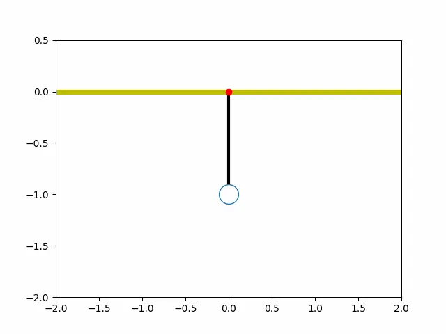
Since the gif file cannot be uploaded in you tube, gif file is uploaded here.

Explanation:

1. Importing Libraries

import numpy as np
from scipy.integrate import odeint
import matplotlib.pyplot as plt
import math
from PIL import Image
import glob

• numpy: Used for numerical computations.
• odeint (from scipy.integrate): Solves differential equations.
• matplotlib.pyplot: For plotting graphs.
• math: For trigonometric functions.
• PIL.Image: To create an animated GIF.
• glob: To manage image files.

2. Defining the Differential Equation

def model(theta, t, b, g, l, m):
    theta1 = theta[0]  # Angular displacement
    theta2 = theta[1]  # Angular velocity
    dtheta1_dt = theta2
    dtheta2_dt = -(b/m) * theta2 - (g/l) * math.sin(theta1)  # Damped pendulum equation
    return [dtheta1_dt, dtheta2_dt]

This function defines the equations of motion for the damped pendulum:

$$\frac{d\theta_1}{dt} = \theta_2$$ $$\frac{d\theta_2}{dt} = -\frac{b}{m} \theta_2 - \frac{g}{l} \sin(\theta_1)$$

Where:

• $\theta_1$ = Angular displacement
• $\theta_2$ = Angular velocity
• $b$ = Damping coefficient
• $g$ = Gravity
• $l$ = Length of the pendulum
• $m$ = Mass

3. Initializing Parameters

b = 0.05  # Damping coefficient
g = 9.81  # Gravity (m/s^2)
l = 1     # Length of pendulum (m)
m = 0.5   # Mass (kg)

theta_0 = [0, 3]  # Initial condition: [initial angle (radians), initial angular velocity]

• The pendulum starts at 0 radians (hanging down) with an initial velocity of 3 rad/s.
• The damping coefficient b = 0.05 adds resistance (friction).

4. Solving the Differential Equations

t = np.linspace(0, 15, 300)  # Time array (0 to 15 sec, 300 points)
theta = odeint(model, theta_0, t, args=(b, g, l, m))

• t: Generates 300 time steps from 0 to 15 seconds.
• odeint(): Solves the system of differential equations.

5. Plotting Angular Displacement & Velocity

plt.plot(t, theta[:, 0], 'b-', label=r'$\frac{d\theta_1}{dt} = \theta_2$')
plt.plot(t, theta[:, 1], 'r--', label=r'$\frac{d\theta_2}{dt} = -\frac{b}{m} \theta_2 - \frac{g}{l} \sin(\theta_1)$')
plt.ylabel('Angle and Angular Velocity')
plt.xlabel('Time [s]')
plt.legend(loc='best')
plt.show()

• theta[:, 0]: Angular displacement vs. time (blue line).
• theta[:, 1]: Angular velocity vs. time (red dashed line).
• The graph helps visualize how the pendulum's motion decays over time due to damping.

6. Simulating Pendulum Motion

ct = 1
for ang in theta[:, 0]:  # Loop through all angles
    x1, y1 = 0, 0  # Pivot point
    x2 = l * math.sin(ang)  # X-coordinate of pendulum bob
    y2 = -l * math.cos(ang)  # Y-coordinate of pendulum bob

    plt.figure()
    plt.plot([-2.0, 2.0], [0, 0], 'y', linewidth=5)  # Ground line
    plt.plot([x1, x2], [y1, y2], linewidth=3)  # Pendulum rod
    plt.plot(x2, y2, 'o', markersize=20, markerfacecolor='w')  # Pendulum bob
    plt.plot(x1, y1, 'o', markersize=6, markerfacecolor='r')  # Pivot point
    plt.xlim([-2.0, 2.0])
    plt.ylim([-2.0, 0.5])

    filename = f'test{ct:05d}.png'
    plt.savefig(filename)
    plt.close()  # Close the figure to save memory
    ct += 1

What This Does:

• Loops through each angle in theta[:, 0] to generate pendulum frames.
• Calculates the bob's position using: $$x_2 = l \sin(\theta)$$ $$y_2 = -l \cos(\theta)$$
• Saves each frame as an image (test00001.png, test00002.png, etc.).

7. Creating an Animated GIF

frames = []
imgs = sorted(glob.glob("test*.png"))  # Get all images in order
for img in imgs:
    new_frame = Image.open(img)
    frames.append(new_frame)

# Save as GIF
if frames:
    frames[0].save('pendulum_animation.gif', format='GIF',
                   append_images=frames[1:], save_all=True,
                   duration=60, loop=0)

print("GIF saved as 'pendulum_animation.gif'")

1. Finds all images (testXXXXX.png) and sorts them.
2. Opens each image and stores it in a list (frames).
3. Creates a looping GIF (pendulum_animation.gif).